Getting real with virtual threads

By Vadim Filanovsky, Mike Huang, Danny Thomas and Martin Chalupa

Intro

Netflix has an extensive history of using Java as our primary programming language across our vast fleet of microservices. As we pick up newer versions of Java, our JVM Ecosystem team seeks out new language features that can improve the ergonomics and performance of our systems. In a recent article, we detailed how our workloads benefited from switching to generational ZGC as our default garbage collector when we migrated to Java 21. Virtual threads is another feature we are excited to adopt as part of this migration.

For those new to virtual threads, they are described as “lightweight threads that dramatically reduce the effort of writing, maintaining, and observing high-throughput concurrent applications.” Their power comes from their ability to be suspended and resumed automatically via continuations when blocking operations occur, thus freeing the underlying operating system threads to be reused for other operations. Leveraging virtual threads can unlock higher performance when utilized in the appropriate context.

In this article we discuss one of the peculiar cases that we encountered along our path to deploying virtual threads on Java 21.

The problem

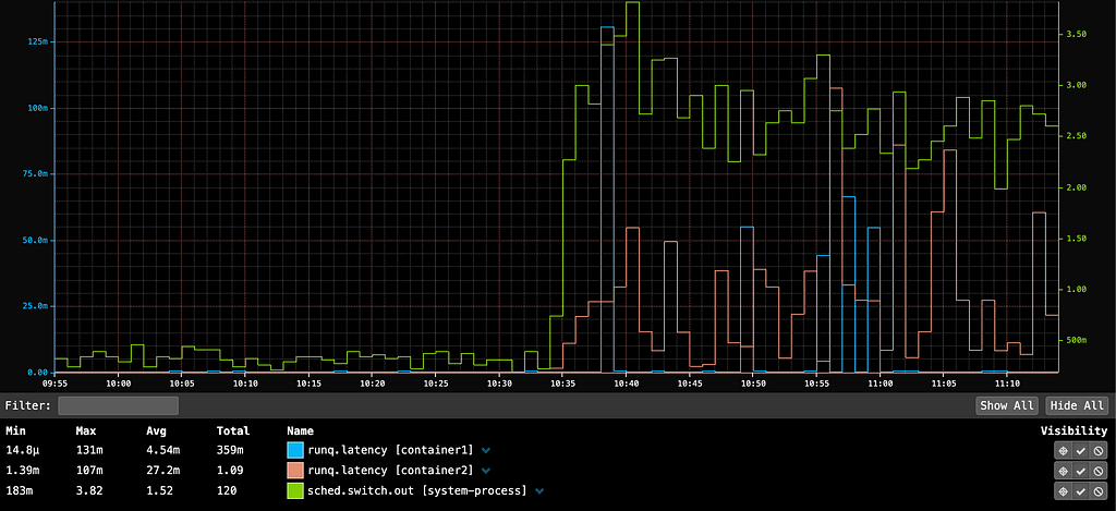
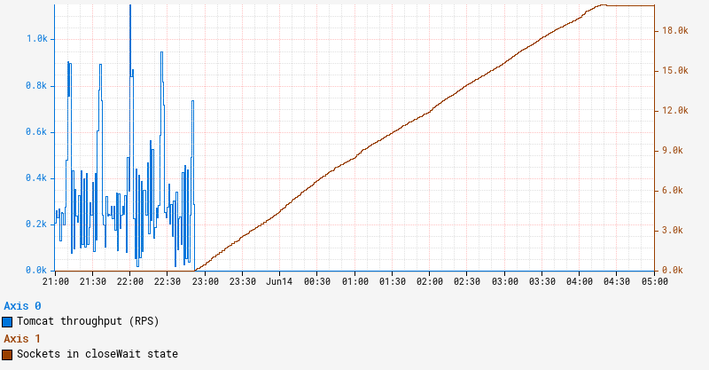
Netflix engineers raised several independent reports of intermittent timeouts and hung instances to the Performance Engineering and JVM Ecosystem teams. Upon closer examination, we noticed a set of common traits and symptoms. In all cases, the apps affected ran on Java 21 with SpringBoot 3 and embedded Tomcat serving traffic on REST endpoints. The instances that experienced the issue simply stopped serving traffic even though the JVM on those instances remained up and running. One clear symptom characterizing the onset of this issue is a persistent increase in the number of sockets in closeWait state as illustrated by the graph below:

Collected diagnostics

Sockets remaining in closeWait state indicate that the remote peer closed the socket, but it was never closed on the local instance, presumably because the application failed to do so. This can often indicate that the application is hanging in an abnormal state, in which case application thread dumps may reveal additional insight.

In order to troubleshoot this issue, we first leveraged our alerts system to catch an instance in this state. Since we periodically collect and persist thread dumps for all JVM workloads, we can often retroactively piece together the behavior by examining these thread dumps from an instance. However, we were surprised to find that all our thread dumps show a perfectly idle JVM with no clear activity. Reviewing recent changes revealed that these impacted services enabled virtual threads, and we knew that virtual thread call stacks do not show up in jstack-generated thread dumps. To obtain a more complete thread dump containing the state of the virtual threads, we used the “jcmd Thread.dump_to_file” command instead. As a last-ditch effort to introspect the state of JVM, we also collected a heap dump from the instance.

Analysis

Thread dumps revealed thousands of “blank” virtual threads:

#119821 "" virtual

#119820 "" virtual

#119823 "" virtual

#120847 "" virtual

#119822 "" virtual
...

These are the VTs (virtual threads) for which a thread object is created, but has not started running, and as such, has no stack trace. In fact, there were approximately the same number of blank VTs as the number of sockets in closeWait state. To make sense of what we were seeing, we need to first understand how VTs operate.

A virtual thread is not mapped 1:1 to a dedicated OS-level thread. Rather, we can think of it as a task that is scheduled to a fork-join thread pool. When a virtual thread enters a blocking call, like waiting for a Future, it relinquishes the OS thread it occupies and simply remains in memory until it is ready to resume. In the meantime, the OS thread can be reassigned to execute other VTs in the same fork-join pool. This allows us to multiplex a lot of VTs to just a handful of underlying OS threads. In JVM terminology, the underlying OS thread is referred to as the “carrier thread” to which a virtual thread can be “mounted” while it executes and “unmounted” while it waits. A great in-depth description of virtual thread is available in JEP 444.

In our environment, we utilize a blocking model for Tomcat, which in effect holds a worker thread for the lifespan of a request. By enabling virtual threads, Tomcat switches to virtual execution. Each incoming request creates a new virtual thread that is simply scheduled as a task on a Virtual Thread Executor. We can see Tomcat creates a VirtualThreadExecutor here.

Tying this information back to our problem, the symptoms correspond to a state when Tomcat keeps creating a new web worker VT for each incoming request, but there are no available OS threads to mount them onto.

Why is Tomcat stuck?

What happened to our OS threads and what are they busy with? As described here, a VT will be pinned to the underlying OS thread if it performs a blocking operation while inside a synchronized block or method. This is exactly what is happening here. Here is a relevant snippet from a thread dump obtained from the stuck instance:

#119515 "" virtual
      java.base/jdk.internal.misc.Unsafe.park(Native Method)
      java.base/java.lang.VirtualThread.parkOnCarrierThread(VirtualThread.java:661)
      java.base/java.lang.VirtualThread.park(VirtualThread.java:593)
      java.base/java.lang.System$2.parkVirtualThread(System.java:2643)
      java.base/jdk.internal.misc.VirtualThreads.park(VirtualThreads.java:54)
      java.base/java.util.concurrent.locks.LockSupport.park(LockSupport.java:219)
      java.base/java.util.concurrent.locks.AbstractQueuedSynchronizer.acquire(AbstractQueuedSynchronizer.java:754)
      java.base/java.util.concurrent.locks.AbstractQueuedSynchronizer.acquire(AbstractQueuedSynchronizer.java:990)
      java.base/java.util.concurrent.locks.ReentrantLock$Sync.lock(ReentrantLock.java:153)
      java.base/java.util.concurrent.locks.ReentrantLock.lock(ReentrantLock.java:322)
      zipkin2.reporter.internal.CountBoundedQueue.offer(CountBoundedQueue.java:54)
      zipkin2.reporter.internal.AsyncReporter$BoundedAsyncReporter.report(AsyncReporter.java:230)
      zipkin2.reporter.brave.AsyncZipkinSpanHandler.end(AsyncZipkinSpanHandler.java:214)
      brave.internal.handler.NoopAwareSpanHandler$CompositeSpanHandler.end(NoopAwareSpanHandler.java:98)
      brave.internal.handler.NoopAwareSpanHandler.end(NoopAwareSpanHandler.java:48)
      brave.internal.recorder.PendingSpans.finish(PendingSpans.java:116)
      brave.RealSpan.finish(RealSpan.java:134)
      brave.RealSpan.finish(RealSpan.java:129)
      io.micrometer.tracing.brave.bridge.BraveSpan.end(BraveSpan.java:117)
      io.micrometer.tracing.annotation.AbstractMethodInvocationProcessor.after(AbstractMethodInvocationProcessor.java:67)
      io.micrometer.tracing.annotation.ImperativeMethodInvocationProcessor.proceedUnderSynchronousSpan(ImperativeMethodInvocationProcessor.java:98)
      io.micrometer.tracing.annotation.ImperativeMethodInvocationProcessor.process(ImperativeMethodInvocationProcessor.java:73)
      io.micrometer.tracing.annotation.SpanAspect.newSpanMethod(SpanAspect.java:59)
      java.base/jdk.internal.reflect.DirectMethodHandleAccessor.invoke(DirectMethodHandleAccessor.java:103)
      java.base/java.lang.reflect.Method.invoke(Method.java:580)
      org.springframework.aop.aspectj.AbstractAspectJAdvice.invokeAdviceMethodWithGivenArgs(AbstractAspectJAdvice.java:637)
...

In this stack trace, we enter the synchronization in brave.RealSpan.finish(RealSpan.java:134). This virtual thread is effectively pinned — it is mounted to an actual OS thread even while it waits to acquire a reentrant lock. There are 3 VTs in this exact state and another VT identified as “<redacted> @DefaultExecutor - 46542” that also follows the same code path. These 4 virtual threads are pinned while waiting to acquire a lock. Because the app is deployed on an instance with 4 vCPUs, the fork-join pool that underpins VT execution also contains 4 OS threads. Now that we have exhausted all of them, no other virtual thread can make any progress. This explains why Tomcat stopped processing the requests and why the number of sockets in closeWait state keeps climbing. Indeed, Tomcat accepts a connection on a socket, creates a request along with a virtual thread, and passes this request/thread to the executor for processing. However, the newly created VT cannot be scheduled because all of the OS threads in the fork-join pool are pinned and never released. So these newly created VTs are stuck in the queue, while still holding the socket.

Who has the lock?

Now that we know VTs are waiting to acquire a lock, the next question is: Who holds the lock? Answering this question is key to understanding what triggered this condition in the first place. Usually a thread dump indicates who holds the lock with either “- locked <0x…> (at …)” or “Locked ownable synchronizers,” but neither of these show up in our thread dumps. As a matter of fact, no locking/parking/waiting information is included in the jcmd-generated thread dumps. This is a limitation in Java 21 and will be addressed in the future releases. Carefully combing through the thread dump reveals that there are a total of 6 threads contending for the same ReentrantLock and associated Condition. Four of these six threads are detailed in the previous section. Here is another thread:

#119516 "" virtual
      java.base/java.lang.VirtualThread.park(VirtualThread.java:582)
      java.base/java.lang.System$2.parkVirtualThread(System.java:2643)
      java.base/jdk.internal.misc.VirtualThreads.park(VirtualThreads.java:54)
      java.base/java.util.concurrent.locks.LockSupport.park(LockSupport.java:219)
      java.base/java.util.concurrent.locks.AbstractQueuedSynchronizer.acquire(AbstractQueuedSynchronizer.java:754)
      java.base/java.util.concurrent.locks.AbstractQueuedSynchronizer.acquire(AbstractQueuedSynchronizer.java:990)
      java.base/java.util.concurrent.locks.ReentrantLock$Sync.lock(ReentrantLock.java:153)
      java.base/java.util.concurrent.locks.ReentrantLock.lock(ReentrantLock.java:322)
      zipkin2.reporter.internal.CountBoundedQueue.offer(CountBoundedQueue.java:54)
      zipkin2.reporter.internal.AsyncReporter$BoundedAsyncReporter.report(AsyncReporter.java:230)
      zipkin2.reporter.brave.AsyncZipkinSpanHandler.end(AsyncZipkinSpanHandler.java:214)
      brave.internal.handler.NoopAwareSpanHandler$CompositeSpanHandler.end(NoopAwareSpanHandler.java:98)
      brave.internal.handler.NoopAwareSpanHandler.end(NoopAwareSpanHandler.java:48)
      brave.internal.recorder.PendingSpans.finish(PendingSpans.java:116)
      brave.RealScopedSpan.finish(RealScopedSpan.java:64)
      ...

Note that while this thread seemingly goes through the same code path for finishing a span, it does not go through a synchronized block. Finally here is the 6th thread:

#107 "AsyncReporter <redacted>"
      java.base/jdk.internal.misc.Unsafe.park(Native Method)
      java.base/java.util.concurrent.locks.LockSupport.park(LockSupport.java:221)
      java.base/java.util.concurrent.locks.AbstractQueuedSynchronizer.acquire(AbstractQueuedSynchronizer.java:754)
      java.base/java.util.concurrent.locks.AbstractQueuedSynchronizer$ConditionObject.awaitNanos(AbstractQueuedSynchronizer.java:1761)
      zipkin2.reporter.internal.CountBoundedQueue.drainTo(CountBoundedQueue.java:81)
      zipkin2.reporter.internal.AsyncReporter$BoundedAsyncReporter.flush(AsyncReporter.java:241)
      zipkin2.reporter.internal.AsyncReporter$Flusher.run(AsyncReporter.java:352)
      java.base/java.lang.Thread.run(Thread.java:1583)

This is actually a normal platform thread, not a virtual thread. Paying particular attention to the line numbers in this stack trace, it is peculiar that the thread seems to be blocked within the internal acquire() method after completing the wait. In other words, this calling thread owned the lock upon entering awaitNanos(). We know the lock was explicitly acquired here. However, by the time the wait completed, it could not reacquire the lock. Summarizing our thread dump analysis:

There are 5 virtual threads and 1 regular thread waiting for the lock. Out of those 5 VTs, 4 of them are pinned to the OS threads in the fork-join pool. There’s still no information on who owns the lock. As there’s nothing more we can glean from the thread dump, our next logical step is to peek into the heap dump and introspect the state of the lock.

Inspecting the lock

Finding the lock in the heap dump was relatively straightforward. Using the excellent Eclipse MAT tool, we examined the objects on the stack of the AsyncReporter non-virtual thread to identify the lock object. Reasoning about the current state of the lock was perhaps the trickiest part of our investigation. Most of the relevant code can be found in the AbstractQueuedSynchronizer.java. While we don’t claim to fully understand the inner workings of it, we reverse-engineered enough of it to match against what we see in the heap dump. This diagram illustrates our findings:

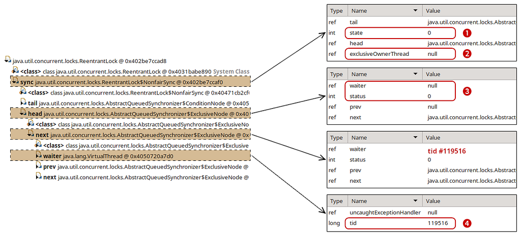
First off, the exclusiveOwnerThread field is null (2), signifying that no one owns the lock. We have an “empty” ExclusiveNode (3) at the head of the list (waiter is null and status is cleared) followed by another ExclusiveNode with waiter pointing to one of the virtual threads contending for the lock — #119516 (4). The only place we found that clears the exclusiveOwnerThread field is within the ReentrantLock.Sync.tryRelease() method (source link). There we also set state = 0 matching the state that we see in the heap dump (1).

With this in mind, we traced the code path to release() the lock. After successfully calling tryRelease(), the lock-holding thread attempts to signal the next waiter in the list. At this point, the lock-holding thread is still at the head of the list, even though ownership of the lock is effectively released. The next node in the list points to the thread that is about to acquire the lock.

To understand how this signaling works, let’s look at the lock acquire path in the AbstractQueuedSynchronizer.acquire() method. Grossly oversimplifying, it’s an infinite loop, where threads attempt to acquire the lock and then park if the attempt was unsuccessful:

while(true) {
   if (tryAcquire()) {
      return; // lock acquired
   }
   park();
}

When the lock-holding thread releases the lock and signals to unpark the next waiter thread, the unparked thread iterates through this loop again, giving it another opportunity to acquire the lock. Indeed, our thread dump indicates that all of our waiter threads are parked on line 754. Once unparked, the thread that managed to acquire the lock should end up in this code block, effectively resetting the head of the list and clearing the reference to the waiter.

To restate this more concisely, the lock-owning thread is referenced by the head node of the list. Releasing the lock notifies the next node in the list while acquiring the lock resets the head of the list to the current node. This means that what we see in the heap dump reflects the state when one thread has already released the lock but the next thread has yet to acquire it. It’s a weird in-between state that should be transient, but our JVM is stuck here. We know thread #119516 was notified and is about to acquire the lock because of the ExclusiveNode state we identified at the head of the list. However, thread dumps show that thread #119516 continues to wait, just like other threads contending for the same lock. How can we reconcile what we see between the thread and heap dumps?

The lock with no place to run

Knowing that thread #119516 was actually notified, we went back to the thread dump to re-examine the state of the threads. Recall that we have 6 total threads waiting for the lock with 4 of the virtual threads each pinned to an OS thread. These 4 will not yield their OS thread until they acquire the lock and proceed out of the synchronized block. #107 “AsyncReporter <redacted>” is a regular platform thread, so nothing should prevent it from proceeding if it acquires the lock. This leaves us with the last thread: #119516. It is a VT, but it is not pinned to an OS thread. Even if it’s notified to be unparked, it cannot proceed because there are no more OS threads left in the fork-join pool to schedule it onto. That’s exactly what happens here — although #119516 is signaled to unpark itself, it cannot leave the parked state because the fork-join pool is occupied by the 4 other VTs waiting to acquire the same lock. None of those pinned VTs can proceed until they acquire the lock. It’s a variation of the classic deadlock problem, but instead of 2 locks we have one lock and a semaphore with 4 permits as represented by the fork-join pool.

Now that we know exactly what happened, it was easy to come up with a reproducible test case.

Conclusion

Virtual threads are expected to improve performance by reducing overhead related to thread creation and context switching. Despite some sharp edges as of Java 21, virtual threads largely deliver on their promise. In our quest for more performant Java applications, we see further virtual thread adoption as a key towards unlocking that goal. We look forward to Java 23 and beyond, which brings a wealth of upgrades and hopefully addresses the integration between virtual threads and locking primitives.

This exploration highlights just one type of issue that performance engineers solve at Netflix. We hope this glimpse into our problem-solving approach proves valuable to others in their future investigations.

Java 21 Virtual Threads - Dude, Where’s My Lock? was originally published in Netflix TechBlog on Medium, where people are continuing the conversation by highlighting and responding to this story.

Hechao Li, Roger Cruz

Cloud Networking Topology

Netflix operates a highly efficient cloud computing infrastructure that supports a wide array of applications essential for our SVOD (Subscription Video on Demand), live streaming and gaming services. Utilizing Amazon AWS, our infrastructure is hosted across multiple geographic regions worldwide. This global distribution allows our applications to deliver content more effectively by serving traffic closer to our customers. Like any distributed system, our applications occasionally require data synchronization between regions to maintain seamless service delivery.

The following diagram shows a simplified cloud network topology for cross-region traffic.

The Problem At First Glance

Our Cloud Network Engineering on-call team received a request to address a network issue affecting an application with cross-region traffic. Initially, it appeared that the application was experiencing timeouts, likely due to suboptimal network performance. As we all know, the longer the network path, the more devices the packets traverse, increasing the likelihood of issues. For this incident, the client application is located in an internal subnet in the US region while the server application is located in an external subnet in a European region. Therefore, it is natural to blame the network since packets need to travel long distances through the internet.

As network engineers, our initial reaction when the network is blamed is typically, “No, it can’t be the network,” and our task is to prove it. Given that there were no recent changes to the network infrastructure and no reported AWS issues impacting other applications, the on-call engineer suspected a noisy neighbor issue and sought assistance from the Host Network Engineering team.

Blame the Neighbors

In this context, a noisy neighbor issue occurs when a container shares a host with other network-intensive containers. These noisy neighbors consume excessive network resources, causing other containers on the same host to suffer from degraded network performance. Despite each container having bandwidth limitations, oversubscription can still lead to such issues.

Upon investigating other containers on the same host — most of which were part of the same application — we quickly eliminated the possibility of noisy neighbors. The network throughput for both the problematic container and all others was significantly below the set bandwidth limits. We attempted to resolve the issue by removing these bandwidth limits, allowing the application to utilize as much bandwidth as necessary. However, the problem persisted.

Blame the Network

We observed some TCP packets in the network marked with the RST flag, a flag indicating that a connection should be immediately terminated. Although the frequency of these packets was not alarmingly high, the presence of any RST packets still raised suspicion on the network. To determine whether this was indeed a network-induced issue, we conducted a tcpdump on the client. In the packet capture file, we spotted one TCP stream that was closed after exactly 30 seconds.

SYN at 18:47:06

After the 3-way handshake (SYN,SYN-ACK,ACK), the traffic started flowing normally. Nothing strange until FIN at 18:47:36 (30 seconds later)

The packet capture results clearly indicated that it was the client application that initiated the connection termination by sending a FIN packet. Following this, the server continued to send data; however, since the client had already decided to close the connection, it responded with RST packets to all subsequent data from the server.

To ensure that the client wasn’t closing the connection due to packet loss, we also conducted a packet capture on the server side to verify that all packets sent by the server were received. This task was complicated by the fact that the packets passed through a NAT gateway (NGW), which meant that on the server side, the client’s IP and port appeared as those of the NGW, differing from those seen on the client side. Consequently, to accurately match TCP streams, we needed to identify the TCP stream on the client side, locate the raw TCP sequence number, and then use this number as a filter on the server side to find the corresponding TCP stream.

With packet capture results from both the client and server sides, we confirmed that all packets sent by the server were correctly received before the client sent a FIN.

Now, from the network point of view, the story is clear. The client initiated the connection requesting data from the server. The server kept sending data to the client with no problem. However, at a certain point, despite the server still having data to send, the client chose to terminate the reception of data. This led us to suspect that the issue might be related to the client application itself.

Blame the Application

In order to fully understand the problem, we now need to understand how the application works. As shown in the diagram below, the application runs in the us-east-1 region. It reads data from cross-region servers and writes the data to consumers within the same region. The client runs as containers, whereas the servers are EC2 instances.

Notably, the cross-region read was problematic while the write path was smooth. Most importantly, there is a 30-second application-level timeout for reading the data. The application (client) errors out if it fails to read an initial batch of data from the servers within 30 seconds. When we increased this timeout to 60 seconds, everything worked as expected. This explains why the client initiated a FIN — because it lost patience waiting for the server to transfer data.

Could it be that the server was updated to send data more slowly? Could it be that the client application was updated to receive data more slowly? Could it be that the data volume became too large to be completely sent out within 30 seconds? Sadly, we received negative answers for all 3 questions from the application owner. The server had been operating without changes for over a year, there were no significant updates in the latest rollout of the client, and the data volume had remained consistent.

Blame the Kernel

If both the network and the application weren’t changed recently, then what changed? In fact, we discovered that the issue coincided with a recent Linux kernel upgrade from version 6.5.13 to 6.6.10. To test this hypothesis, we rolled back the kernel upgrade and it did restore normal operation to the application.

Honestly speaking, at that time I didn’t believe it was a kernel bug because I assumed the TCP implementation in the kernel should be solid and stable (Spoiler alert: How wrong was I!). But we were also out of ideas from other angles.

There were about 14k commits between the good and bad kernel versions. Engineers on the team methodically and diligently bisected between the two versions. When the bisecting was narrowed to a couple of commits, a change with “tcp” in its commit message caught our attention. The final bisecting confirmed that this commit was our culprit.

Interestingly, while reviewing the email history related to this commit, we found that another user had reported a Python test failure following the same kernel upgrade. Although their solution was not directly applicable to our situation, it suggested that a simpler test might also reproduce our problem. Using strace, we observed that the application configured the following socket options when communicating with the server:

[pid 1699] setsockopt(917, SOL_IPV6, IPV6_V6ONLY, [0], 4) = 0
[pid 1699] setsockopt(917, SOL_SOCKET, SO_KEEPALIVE, [1], 4) = 0
[pid 1699] setsockopt(917, SOL_SOCKET, SO_SNDBUF, [131072], 4) = 0
[pid 1699] setsockopt(917, SOL_SOCKET, SO_RCVBUF, [65536], 4) = 0
[pid 1699] setsockopt(917, SOL_TCP, TCP_NODELAY, [1], 4) = 0

We then developed a minimal client-server C application that transfers a file from the server to the client, with the client configuring the same set of socket options. During testing, we used a 10M file, which represents the volume of data typically transferred within 30 seconds before the client issues a FIN. On the old kernel, this cross-region transfer completed in 22 seconds, whereas on the new kernel, it took 39 seconds to finish.

The Root Cause

With the help of the minimal reproduction setup, we were ultimately able to pinpoint the root cause of the problem. In order to understand the root cause, it’s essential to have a grasp of the TCP receive window.

TCP Receive Window

Simply put, the TCP receive window is how the receiver tells the sender “This is how many bytes you can send me without me ACKing any of them”. Assuming the sender is the server and the receiver is the client, then we have:

The Window Size

Now that we know the TCP receive window size could affect the throughput, the question is, how is the window size calculated? As an application writer, you can’t decide the window size, however, you can decide how much memory you want to use for buffering received data. This is configured using SO_RCVBUF socket option we saw in the strace result above. However, note that the value of this option means how much application data can be queued in the receive buffer. In man 7 socket, there is

SO_RCVBUF

Sets or gets the maximum socket receive buffer in bytes.
The kernel doubles this value (to allow space for
bookkeeping overhead) when it is set using setsockopt(2),
and this doubled value is returned by getsockopt(2). The
default value is set by the
/proc/sys/net/core/rmem_default file, and the maximum
allowed value is set by the /proc/sys/net/core/rmem_max
file. The minimum (doubled) value for this option is 256.

This means, when the user gives a value X, then the kernel stores 2X in the variable sk->sk_rcvbuf. In other words, the kernel assumes that the bookkeeping overhead is as much as the actual data (i.e. 50% of the sk_rcvbuf).

sysctl_tcp_adv_win_scale

However, the assumption above may not be true because the actual overhead really depends on a lot of factors such as Maximum Transmission Unit (MTU). Therefore, the kernel provided this sysctl_tcp_adv_win_scale which you can use to tell the kernel what the actual overhead is. (I believe 99% of people also don’t know how to set this parameter correctly and I’m definitely one of them. You’re the kernel, if you don’t know the overhead, how can you expect me to know?).

According to the sysctl doc,

tcp_adv_win_scale — INTEGER

Obsolete since linux-6.6 Count buffering overhead as bytes/2^tcp_adv_win_scale (if tcp_adv_win_scale > 0) or bytes-bytes/2^(-tcp_adv_win_scale), if it is <= 0.

Possible values are [-31, 31], inclusive.

Default: 1

For 99% of people, we’re just using the default value 1, which in turn means the overhead is calculated by rcvbuf/2^tcp_adv_win_scale = 1/2 * rcvbuf. This matches the assumption when setting the SO_RCVBUF value.

Let’s recap. Assume you set SO_RCVBUF to 65536, which is the value set by the application as shown in the setsockopt syscall. Then we have:

• SO_RCVBUF = 65536
• rcvbuf = 2 * 65536 = 131072
• overhead = rcvbuf / 2 = 131072 / 2 = 65536
• receive window size = rcvbuf — overhead = 131072–65536 = 65536

(Note, this calculation is simplified. The real calculation is more complex.)

In short, the receive window size before the kernel upgrade was 65536. With this window size, the application was able to transfer 10M data within 30 seconds.

The Change

This commit obsoleted sysctl_tcp_adv_win_scale and introduced a scaling_ratio that can more accurately calculate the overhead or window size, which is the right thing to do. With the change, the window size is now rcvbuf * scaling_ratio.

So how is scaling_ratio calculated? It is calculated using skb->len/skb->truesize where skb->len is the length of the tcp data length in an skb and truesize is the total size of the skb. This is surely a more accurate ratio based on real data rather than a hardcoded 50%. Now, here is the next question: during the TCP handshake before any data is transferred, how do we decide the initial scaling_ratio? The answer is, a magic and conservative ratio was chosen with the value being roughly 0.25.

Now we have:

• SO_RCVBUF = 65536
• rcvbuf = 2 * 65536 = 131072
• receive window size = rcvbuf * 0.25 = 131072 * 0.25 = 32768

In short, the receive window size halved after the kernel upgrade. Hence the throughput was cut in half, causing the data transfer time to double.

Naturally, you may ask, I understand that the initial window size is small, but why doesn’t the window grow when we have a more accurate ratio of the payload later (i.e. skb->len/skb->truesize)? With some debugging, we eventually found out that the scaling_ratio does get updated to a more accurate skb->len/skb->truesize, which in our case is around 0.66. However, another variable, window_clamp, is not updated accordingly. window_clamp is the maximum receive window allowed to be advertised, which is also initialized to 0.25 * rcvbuf using the initial scaling_ratio. As a result, the receive window size is capped at this value and can’t grow bigger.

The Fix

In theory, the fix is to update window_clamp along with scaling_ratio. However, in order to have a simple fix that doesn’t introduce other unexpected behaviors, our final fix was to increase the initial scaling_ratio from 25% to 50%. This will make the receive window size backward compatible with the original default sysctl_tcp_adv_win_scale.

Meanwhile, notice that the problem is not only caused by the changed kernel behavior but also by the fact that the application sets SO_RCVBUF and has a 30-second application-level timeout. In fact, the application is Kafka Connect and both settings are the default configurations (receive.buffer.bytes=64k and request.timeout.ms=30s). We also created a kafka ticket to change receive.buffer.bytes to -1 to allow Linux to auto tune the receive window.

Conclusion

This was a very interesting debugging exercise that covered many layers of Netflix’s stack and infrastructure. While it technically wasn’t the “network” to blame, this time it turned out the culprit was the software components that make up the network (i.e. the TCP implementation in the kernel).

If tackling such technical challenges excites you, consider joining our Cloud Infrastructure Engineering teams. Explore opportunities by visiting Netflix Jobs and searching for Cloud Engineering positions.

Acknowledgments

Special thanks to our stunning colleagues Alok Tiagi, Artem Tkachuk, Ethan Adams, Jorge Rodriguez, Nick Mahilani, Tycho Andersen and Vinay Rayini for investigating and mitigating this issue. We would also like to thank Linux kernel network expert Eric Dumazet for reviewing and applying the patch.

Investigation of a Cross-regional Network Performance Issue was originally published in Netflix TechBlog on Medium, where people are continuing the conversation by highlighting and responding to this story.

By Aurélien Bibaut, Winston Chou, Simon Ejdemyr, and Nathan Kallus

We are excited to share our work on how to learn good proxy metrics from historical experiments at KDD 2024. This work addresses a fundamental question for technology companies and academic researchers alike: how do we establish that a treatment that improves short-term (statistically sensitive) outcomes also improves long-term (statistically insensitive) outcomes? Or, faced with multiple short-term outcomes, how do we optimally trade them off for long-term benefit?

For example, in an A/B test, you may observe that a product change improves the click-through rate. However, the test does not provide enough signal to measure a change in long-term retention, leaving you in the dark as to whether this treatment makes users more satisfied with your service. The click-through rate is a proxy metric (S, for surrogate, in our paper) while retention is a downstream business outcome or north star metric (Y). We may even have several proxy metrics, such as other types of clicks or the length of engagement after click. Taken together, these form a vector of proxy metrics.

The goal of our work is to understand the true relationship between the proxy metric(s) and the north star metric — so that we can assess a proxy’s ability to stand in for the north star metric, learn how to combine multiple metrics into a single best one, and better explore and compare different proxies.

Several intuitive approaches to understanding this relationship have surprising pitfalls:

• Looking only at user-level correlations between the proxy S and north star Y. Continuing the example from above, you may find that users with a higher click-through rate also tend to have a higher retention. But this does not mean that a product change that improves the click-through rate will also improve retention (in fact, promoting clickbait may have the opposite effect). This is because, as any introductory causal inference class will tell you, there are many confounders between S and Y — many of which you can never reliably observe and control for.
• Looking naively at treatment effect correlations between S and Y. Suppose you are lucky enough to have many historical A/B tests. Further imagine the ordinary least squares (OLS) regression line through a scatter plot of Y on S in which each point represents the (S,Y)-treatment effect from a previous test. Even if you find that this line has a positive slope, you unfortunately cannot conclude that product changes that improve S will also improve Y. The reason for this is correlated measurement error — if S and Y are positively correlated in the population, then treatment arms that happen to have more users with high S will also have more users with high Y.

Between these naive approaches, we find that the second one is the easier trap to fall into. This is because the dangers of the first approach are well-known, whereas covariances between estimated treatment effects can appear misleadingly causal. In reality, these covariances can be severely biased compared to what we actually care about: covariances between true treatment effects. In the extreme — such as when the negative effects of clickbait are substantial but clickiness and retention are highly correlated at the user level — the true relationship between S and Y can be negative even if the OLS slope is positive. Only more data per experiment could diminish this bias — using more experiments as data points will only yield more precise estimates of the badly biased slope. At first glance, this would appear to imperil any hope of using existing experiments to detect the relationship.

To overcome this bias, we propose better ways to leverage historical experiments, inspired by techniques from the literature on weak instrumental variables. More specifically, we show that three estimators are consistent for the true proxy/north-star relationship under different constraints (the paper provides more details and should be helpful for practitioners interested in choosing the best estimator for their setting):

• A Total Covariance (TC) estimator allows us to estimate the OLS slope from a scatter plot of true treatment effects by subtracting the scaled measurement error covariance from the covariance of estimated treatment effects. Under the assumption that the correlated measurement error is the same across experiments (homogeneous covariances), the bias of this estimator is inversely proportional to the total number of units across all experiments, as opposed to the number of members per experiment.
• Jackknife Instrumental Variables Estimation (JIVE) converges to the same OLS slope as the TC estimator but does not require the assumption of homogeneous covariances. JIVE eliminates correlated measurement error by removing each observation’s data from the computation of its instrumented surrogate values.
• A Limited Information Maximum Likelihood (LIML) estimator is statistically efficient as long as there are no direct effects between the treatment and Y (that is, S fully mediates all treatment effects on Y). We find that LIML is highly sensitive to this assumption and recommend TC or JIVE for most applications.

Our methods yield linear structural models of treatment effects that are easy to interpret. As such, they are well-suited to the decentralized and rapidly-evolving practice of experimentation at Netflix, which runs thousands of experiments per year on many diverse parts of the business. Each area of experimentation is staffed by independent Data Science and Engineering teams. While every team ultimately cares about the same north star metrics (e.g., long-term revenue), it is highly impractical for most teams to measure these in short-term A/B tests. Therefore, each has also developed proxies that are more sensitive and directly relevant to their work (e.g., user engagement or latency). To complicate matters more, teams are constantly innovating on these secondary metrics to find the right balance of sensitivity and long-term impact.

In this decentralized environment, linear models of treatment effects are a highly useful tool for coordinating efforts around proxy metrics and aligning them towards the north star:

1. Managing metric tradeoffs. Because experiments in one area can affect metrics in another area, there is a need to measure all secondary metrics in all tests, but also to understand the relative impact of these metrics on the north star. This is so we can inform decision-making when one metric trades off against another metric.
2. Informing metrics innovation. To minimize wasted effort on metric development, it is also important to understand how metrics correlate with the north star “net of” existing metrics.
3. Enabling teams to work independently. Lastly, teams need simple tools in order to iterate on their own metrics. Teams may come up with dozens of variations of secondary metrics, and slow, complicated tools for evaluating these variations are unlikely to be adopted. Conversely, our models are easy and fast to fit, and are actively used to develop proxy metrics at Netflix.

We are thrilled about the research and implementation of these methods at Netflix — while also continuing to strive for great and always better, per our culture. For example, we still have some way to go to develop a more flexible data architecture to streamline the application of these methods within Netflix. Interested in helping us? See our open job postings!

For feedback on this blog post and for supporting and making this work better, we thank Apoorva Lal, Martin Tingley, Patric Glynn, Richard McDowell, Travis Brooks, and Ayal Chen-Zion.

Improve Your Next Experiment by Learning Better Proxy Metrics From Past Experiments was originally published in Netflix TechBlog on Medium, where people are continuing the conversation by highlighting and responding to this story.

By Jiangwei Pan, Gary Tang, Henry Wang, and Justin Basilico

Introduction

Our mission at Netflix is to entertain the world. Our personalization algorithms play a crucial role in delivering on this mission for all members by recommending the right shows, movies, and games at the right time. This goal extends beyond immediate engagement; we aim to create an experience that brings lasting enjoyment to our members. Traditional recommender systems often optimize for short-term metrics like clicks or engagement, which may not fully capture long-term satisfaction. We strive to recommend content that not only engages members in the moment but also enhances their long-term satisfaction, which increases the value they get from Netflix, and thus they’ll be more likely to continue to be a member.

Recommendations as Contextual Bandit

One simple way we can view recommendations is as a contextual bandit problem. When a member visits, that becomes a context for our system and it selects an action of what recommendations to show, and then the member provides various types of feedback. These feedback signals can be immediate (skips, plays, thumbs up/down, or adding items to their playlist) or delayed (completing a show or renewing their subscription). We can define reward functions to reflect the quality of the recommendations from these feedback signals and then train a contextual bandit policy on historical data to maximize the expected reward.

Improving Recommendations: Models and Objectives

There are many ways that a recommendation model can be improved. They may come from more informative input features, more data, different architectures, more parameters, and so forth. In this post, we focus on a less-discussed aspect about improving the recommender objective by defining a reward function that tries to better reflect long-term member satisfaction.

Retention as Reward?

Member retention might seem like an obvious reward for optimizing long-term satisfaction because members should stay if they’re satisfied, however it has several drawbacks:

• Noisy: Retention can be influenced by numerous external factors, such as seasonal trends, marketing campaigns, or personal circumstances unrelated to the service.
• Low Sensitivity: Retention is only sensitive for members on the verge of canceling their subscription, not capturing the full spectrum of member satisfaction.
• Hard to Attribute: Members might cancel only after a series of bad recommendations.
• Slow to Measure: We only get one signal per account per month.

Due to these challenges, optimizing for retention alone is impractical.

Proxy Rewards

Instead, we can train our bandit policy to optimize a proxy reward function that is highly aligned with long-term member satisfaction while being sensitive to individual recommendations. The proxy reward r(user, item) is a function of user interaction with the recommended item. For example, if we recommend “One Piece” and a member plays then subsequently completes and gives it a thumbs-up, a simple proxy reward might be defined as r(user, item) = f(play, complete, thumb).

Click-through rate (CTR)

Click-through rate (CTR), or in our case play-through rate, can be viewed as a simple proxy reward where r(user, item) = 1 if the user clicks a recommendation and 0 otherwise. CTR is a common feedback signal that generally reflects user preference expectations. It is a simple yet strong baseline for many recommendation applications. In some cases, such as ads personalization where the click is the target action, CTR may even be a reasonable reward for production models. However, in most cases, over-optimizing CTR can lead to promoting clickbaity items, which may harm long-term satisfaction.

Beyond CTR

To align the proxy reward function more closely with long-term satisfaction, we need to look beyond simple interactions, consider all types of user actions, and understand their true implications on user satisfaction.

We give a few examples in the Netflix context:

• Fast season completion ✅: Completing a season of a recommended TV show in one day is a strong sign of enjoyment and long-term satisfaction.
• Thumbs-down after completion ❌: Completing a TV show in several weeks followed by a thumbs-down indicates low satisfaction despite significant time spent.
• Playing a movie for just 10 minutes ❓: In this case, the user’s satisfaction is ambiguous. The brief engagement might indicate that the user decided to abandon the movie, or it could simply mean the user was interrupted and plans to finish the movie later, perhaps the next day.
• Discovering new genres ✅ ✅: Watching more Korean or game shows after “Squid Game” suggests the user is discovering something new. This discovery was likely even more valuable since it led to a variety of engagements in a new area for a member.

Reward Engineering

Reward engineering is the iterative process of refining the proxy reward function to align with long-term member satisfaction. It is similar to feature engineering, except that it can be derived from data that isn’t available at serving time. Reward engineering involves four stages: hypothesis formation, defining a new proxy reward, training a new bandit policy, and A/B testing. Below is a simple example.

Challenge: Delayed Feedback

User feedback used in the proxy reward function is often delayed or missing. For example, a member may decide to play a recommended show for just a few minutes on the first day and take several weeks to fully complete the show. This completion feedback is therefore delayed. Additionally, some user feedback may never occur; while we may wish otherwise, not all members provide a thumbs-up or thumbs-down after completing a show, leaving us uncertain about their level of enjoyment.

We could try and wait to give a longer window to observe feedback, but how long should we wait for delayed feedback before computing the proxy rewards? If we wait too long (e.g., weeks), we miss the opportunity to update the bandit policy with the latest data. In a highly dynamic environment like Netflix, a stale bandit policy can degrade the user experience and be particularly bad at recommending newer items.

Solution: predict missing feedback

We aim to update the bandit policy shortly after making a recommendation while also defining the proxy reward function based on all user feedback, including delayed feedback. Since delayed feedback has not been observed at the time of policy training, we can predict it. This prediction occurs for each training example with delayed feedback, using already observed feedback and other relevant information up to the training time as input features. Thus, the prediction also gets better as time progresses.

The proxy reward is then calculated for each training example using both observed and predicted feedback. These training examples are used to update the bandit policy.

But aren’t we still only relying on observed feedback in the proxy reward function? Yes, because delayed feedback is predicted based on observed feedback. However, it is simpler to reason about rewards using all feedback directly. For instance, the delayed thumbs-up prediction model may be a complex neural network that takes into account all observed feedback (e.g., short-term play patterns). It’s more straightforward to define the proxy reward as a simple function of the thumbs-up feedback rather than a complex function of short-term interaction patterns. It can also be used to adjust for potential biases in how feedback is provided.

The reward engineering diagram is updated with an optional delayed feedback prediction step.

Two types of ML models

It’s worth noting that this approach employs two types of ML models:

• Delayed Feedback Prediction Models: These models predict p(final feedback | observed feedbacks). The predictions are used to define and compute proxy rewards for bandit policy training examples. As a result, these models are used offline during the bandit policy training.
• Bandit Policy Models: These models are used in the bandit policy π(item | user; r) to generate recommendations online and in real-time.

Challenge: Online-Offline Metric Disparity

Improved input features or neural network architectures often lead to better offline model metrics (e.g., AUC for classification models). However, when these improved models are subjected to A/B testing, we often observe flat or even negative online metrics, which can quantify long-term member satisfaction.

This online-offline metric disparity usually occurs when the proxy reward used in the recommendation policy is not fully aligned with long-term member satisfaction. In such cases, a model may achieve higher proxy rewards (offline metrics) but result in worse long-term member satisfaction (online metrics).

Nevertheless, the model improvement is genuine. One approach to resolve this is to further refine the proxy reward definition to align better with the improved model. When this tuning results in positive online metrics, the model improvement can be effectively productized. See [1] for more discussions on this challenge.

Summary and Open Questions

In this post, we provided an overview of our reward engineering efforts to align Netflix recommendations with long-term member satisfaction. While retention remains our north star, it is not easy to optimize directly. Therefore, our efforts focus on defining a proxy reward that is aligned with long-term satisfaction and sensitive to individual recommendations. Finally, we discussed the unique challenge of delayed user feedback at Netflix and proposed an approach that has proven effective for us. Refer to [2] for an earlier overview of the reward innovation efforts at Netflix.

As we continue to improve our recommendations, several open questions remain:

• Can we learn a good proxy reward function automatically by correlating behavior with retention?
• How long should we wait for delayed feedback before using its predicted value in policy training?
• How can we leverage Reinforcement Learning to further align the policy with long-term satisfaction?

References

[1] Deep learning for recommender systems: A Netflix case study. AI Magazine 2021. Harald Steck, Linas Baltrunas, Ehtsham Elahi, Dawen Liang, Yves Raimond, Justin Basilico.

[2] Reward innovation for long-term member satisfaction. RecSys 2023. Gary Tang, Jiangwei Pan, Henry Wang, Justin Basilico.

Recommending for Long-Term Member Satisfaction at Netflix was originally published in Netflix TechBlog on Medium, where people are continuing the conversation by highlighting and responding to this story.

By Jose Fernandez, Sebastien Dabdoub, Jason Koch, Artem Tkachuk

The Compute and Performance Engineering teams at Netflix regularly investigate performance issues in our multi-tenant environment. The first step is determining whether the problem originates from the application or the underlying infrastructure. One issue that often complicates this process is the "noisy neighbor" problem. On Titus, our multi-tenant compute platform, a "noisy neighbor" refers to a container or system service that heavily utilizes the server's resources, causing performance degradation in adjacent containers. We usually focus on CPU utilization because it is our workloads’ most frequent source of noisy neighbor issues.

Detecting the effects of noisy neighbors is complex. Traditional performance analysis tools such as perf can introduce significant overhead, risking further performance degradation. Additionally, these tools are typically deployed after the fact, which is too late for effective investigation. Another challenge is that debugging noisy neighbor issues requires significant low-level expertise and specialized tooling. In this blog post, we'll reveal how we leveraged eBPF to achieve continuous, low-overhead instrumentation of the Linux scheduler, enabling effective self-serve monitoring of noisy neighbor issues. You’ll learn how Linux kernel instrumentation can improve your infrastructure observability with deeper insights and enhanced monitoring.

Continuous Instrumentation of the Linux Scheduler

To ensure the reliability of our workloads that depend on low latency responses, we instrumented the run queue latency for each container, which measures the time processes spend in the scheduling queue before being dispatched to the CPU. Extended waiting in this queue can be a telltale of performance issues, especially when containers are not utilizing their total CPU allocation. Continuous instrumentation is critical to catching such matters as they emerge, and eBPF, with its hooks into the Linux scheduler with minimal overhead, enabled us to monitor run queue latency efficiently.

To emit a run queue latency metric, we leveraged three eBPF hooks: sched_wakeup, sched_wakeup_new, and sched_switch.

The sched_wakeup and sched_wakeup_new hooks are invoked when a process changes state from 'sleeping' to 'runnable.' They let us identify when a process is ready to run and is waiting for CPU time. During this event, we generate a timestamp and store it in an eBPF hash map using the process ID as the key.

struct {
    __uint(type, BPF_MAP_TYPE_HASH);
    __uint(max_entries, MAX_TASK_ENTRIES);
    __uint(key_size, sizeof(u32));
    __uint(value_size, sizeof(u64));
} runq_enqueued SEC(".maps");

SEC("tp_btf/sched_wakeup")
int tp_sched_wakeup(u64 *ctx)
{
    struct task_struct *task = (void *)ctx[0];
    u32 pid = task->pid;
    u64 ts = bpf_ktime_get_ns();

    bpf_map_update_elem(&runq_enqueued, &pid, &ts, BPF_NOEXIST);
    return 0;
}

Conversely, the sched_switch hook is triggered when the CPU switches between processes. This hook provides pointers to the process currently utilizing the CPU and the process about to take over. We use the upcoming task's process ID (PID) to fetch the timestamp from the eBPF map. This timestamp represents when the process entered the queue, which we had previously stored. We then calculate the run queue latency by simply subtracting the timestamps.

SEC("tp_btf/sched_switch")
int tp_sched_switch(u64 *ctx)
{
    struct task_struct *prev = (struct task_struct *)ctx[1];
    struct task_struct *next = (struct task_struct *)ctx[2];
    u32 prev_pid = prev->pid;
    u32 next_pid = next->pid;
 
    // fetch timestamp of when the next task was enqueued
    u64 *tsp = bpf_map_lookup_elem(&runq_enqueued, &next_pid);
    if (tsp == NULL) {
        return 0; // missed enqueue
    }

    // calculate runq latency before deleting the stored timestamp
    u64 now = bpf_ktime_get_ns();
    u64 runq_lat = now - *tsp;

    // delete pid from enqueued map
    bpf_map_delete_elem(&runq_enqueued, &next_pid);
    ....

One of the advantages of eBPF is its ability to provide pointers to the actual kernel data structures representing processes or threads, also known as tasks in kernel terminology. This feature enables access to a wealth of information stored about a process. We required the process's cgroup ID to associate it with a container for our specific use case. However, the cgroup information in the process struct is safeguarded by an RCU (Read Copy Update) lock.

To safely access this RCU-protected information, we can leverage kfuncs in eBPF. kfuncs are kernel functions that can be called from eBPF programs. There are kfuncs available to lock and unlock RCU read-side critical sections. These functions ensure that our eBPF program remains safe and efficient while retrieving the cgroup ID from the task struct.

void bpf_rcu_read_lock(void) __ksym;
void bpf_rcu_read_unlock(void) __ksym;

u64 get_task_cgroup_id(struct task_struct *task)
{
    struct css_set *cgroups;
    u64 cgroup_id;
    bpf_rcu_read_lock();
    cgroups = task->cgroups;
    cgroup_id = cgroups->dfl_cgrp->kn->id;
    bpf_rcu_read_unlock();
    return cgroup_id;
}

Once the data is ready, we must package it and send it to userspace. For this purpose, we chose the eBPF ring buffer. It is efficient, high-performing, and user-friendly. It can handle variable-length data records and allows data reading without necessitating extra memory copying or syscalls. However, the sheer number of data points was causing the userspace program to use too much CPU, so we implemented a rate limiter in eBPF to sample the data.

struct {
    __uint(type, BPF_MAP_TYPE_RINGBUF);
    __uint(max_entries, RINGBUF_SIZE_BYTES);
} events SEC(".maps");

struct {
    __uint(type, BPF_MAP_TYPE_PERCPU_HASH);
    __uint(max_entries, MAX_TASK_ENTRIES);
    __uint(key_size, sizeof(u64));
    __uint(value_size, sizeof(u64));
} cgroup_id_to_last_event_ts SEC(".maps");

struct runq_event {
    u64 prev_cgroup_id;
    u64 cgroup_id;
    u64 runq_lat;
    u64 ts;
};

SEC("tp_btf/sched_switch")
int tp_sched_switch(u64 *ctx)
{
    // ....
    // The previous code
    // ....
 
    u64 prev_cgroup_id = get_task_cgroup_id(prev);
    u64 cgroup_id = get_task_cgroup_id(next);
 
    // per-cgroup-id-per-CPU rate-limiting 
    // to balance observability with performance overhead
    u64 *last_ts = 
        bpf_map_lookup_elem(&cgroup_id_to_last_event_ts, &cgroup_id);
    u64 last_ts_val = last_ts == NULL ? 0 : *last_ts;

    // check the rate limit for the cgroup_id in consideration
    // before doing more work
    if (now - last_ts_val < RATE_LIMIT_NS) {
        // Rate limit exceeded, drop the event
        return 0;
    }

    struct runq_event *event;
    event = bpf_ringbuf_reserve(&events, sizeof(*event), 0);
  
    if (event) {
        event->prev_cgroup_id = prev_cgroup_id;
        event->cgroup_id = cgroup_id;
        event->runq_lat = runq_lat;
        event->ts = now;
        bpf_ringbuf_submit(event, 0);
        // Update the last event timestamp for the current cgroup_id
        bpf_map_update_elem(&cgroup_id_to_last_event_ts, &cgroup_id,
            &now, BPF_ANY);

    }

    return 0;
}

Our userspace application, developed in Go, processes events from the ring buffer to emit metrics to our metrics backend, Atlas. Each event includes a run queue latency sample with a cgroup ID, which we associate with containers running on the host. We categorize it as a system service if no such association is found. When a cgroup ID is associated with a container, we emit a percentile timer Atlas metric (runq.latency) for that container. We also increment a counter metric (sched.switch.out) to monitor preemptions occurring for the container's processes. Access to the prev_cgroup_id of the preempted process allows us to tag the metric with the cause of the preemption, whether it's due to a process within the same container (or cgroup), a process in another container, or a system service.

It's important to highlight that both the runq.latency metric and the sched.switch.out metrics are needed to determine if a container is affected by noisy neighbors, which is the goal we aim to achieve — relying solely on the runq.latency metric can lead to misconceptions. For example, if a container is at or over its cgroup CPU limit, the scheduler will throttle it, resulting in an apparent spike in run queue latency due to delays in the queue. If we were only to consider this metric, we might incorrectly attribute the performance degradation to noisy neighbors when it's actually because the container is hitting its CPU quota. However, simultaneous spikes in both metrics, mainly when the cause is a different container or system process, clearly indicate a noisy neighbor issue.

A Noisy Neighbor Story

Below is the runq.latency metric for a server running a single container with ample CPU capacity. The 99th percentile averages 83.4µs (microseconds), serving as our baseline. Although there are some spikes reaching 400µs, the latency remains within acceptable parameters.

At 10:35, launching container2, which fully utilized all CPUs on the host, caused a significant 131-millisecond spike (131,000 microseconds) in container1's P99 run queue latency. This spike would be noticeable in the userspace application if it were serving HTTP traffic. If userspace app owners reported an unexplained latency spike, we could quickly identify the noisy neighbor issue through run queue latency metrics.

The sched.switch.out metric indicates that the spike was due to increased preemptions by system processes, highlighting a noisy neighbor issue where system services compete with containers for CPU time. Our metrics show that the noisy neighbors were actually system processes, likely triggered by container2 consuming all available CPU capacity.

Optimizing eBPF Code

We developed an open-source eBPF process monitoring tool called bpftop to measure the overhead of eBPF code in this kernel hot path. Our profiling with bpftop shows that the instrumentation adds less than 600 nanoseconds to each sched_* hook. We conducted a performance analysis on a Java service running in a container, and the instrumentation did not introduce significant overhead. The performance variance with the run queue profiling code active versus inactive was not measurable in milliseconds.

During our research on how eBPF statistics are measured in the kernel, we identified an opportunity to improve the calculation. We submitted this patch, which was included in the Linux kernel 6.10 release.

Through trial and error and using bpftop, we identified several optimizations that helped maintain low overhead for our eBPF code:

• We found that BPF_MAP_TYPE_HASH was the most performant for storing enqueued timestamps. Using BPF_MAP_TYPE_TASK_STORAGE resulted in nearly a twofold performance decline. BPF_MAP_TYPE_PERCPU_HASH was slightly less performant than BPF_MAP_TYPE_HASH, which was unexpected and requires further investigation.
• BPF_MAP_TYPE_LRU_HASH maps are 40–50 nanoseconds slower per operation than regular hash maps. Due to space concerns from PID churn, we initially used them for enqueued timestamps. Ultimately, we settled on BPF_MAP_TYPE_HASH with an increased size to mitigate this risk.
• The BPF_CORE_READ helper adds 20–30 nanoseconds per invocation. In the case of raw tracepoints, specifically those that are "BTF-enabled" (tp_btf/*), it is safe and more efficient to access the task struct members directly. Andrii Nakryiko recommends this approach in this blog post.
• The sched_switch, sched_wakeup, and sched_wakeup_new are all triggered for kernel tasks, which are identifiable by their PID of 0. We found monitoring these tasks unnecessary, so we implemented several early exit conditions and conditional logic to prevent executing costly operations, such as accessing BPF maps, when dealing with a kernel task. Notably, kernel tasks operate through the scheduler queue like any regular process.

Conclusion

Our findings highlight the value of low-overhead continuous instrumentation of the Linux kernel with eBPF. We have integrated these metrics into customer dashboards, enabling actionable insights and guiding multitenancy performance discussions. We can also now use these metrics to refine CPU isolation strategies to minimize the impact of noisy neighbors. Additionally, thanks to these metrics, we've gained deeper insights into the Linux scheduler.

This work has also deepened our understanding of eBPF technology and underscored the importance of tools like bpftop for optimizing eBPF code. As eBPF adoption increases, we foresee more infrastructure observability and business logic shifting to it. One promising project in this space is sched_ext, which has the potential to revolutionize how scheduling decisions are made and tailored to specific workload needs.

Noisy Neighbor Detection with eBPF was originally published in Netflix TechBlog on Medium, where people are continuing the conversation by highlighting and responding to this story.

By Karthik Yagna, Baskar Odayarkoil, and Alex Ellis

Pushy is Netflix’s WebSocket server that maintains persistent WebSocket connections with devices running the Netflix application. This allows data to be sent to the device from backend services on demand, without the need for continually polling requests from the device. Over the last few years, Pushy has seen tremendous growth, evolving from its role as a best-effort message delivery service to be an integral part of the Netflix ecosystem. This post describes how we’ve grown and scaled Pushy to meet its new and future needs, as it handles hundreds of millions of concurrent WebSocket connections, delivers hundreds of thousands of messages per second, and maintains a steady 99.999% message delivery reliability rate.

History & motivation

There were two main motivating use cases that drove Pushy’s initial development and usage. The first was voice control, where you can play a title or search using your virtual assistant with a voice command like “Show me Stranger Things on Netflix.” (See How to use voice controls with Netflix if you want to do this yourself!).

If we consider the Alexa use case, we can see how this partnership with Amazon enabled this to work. Once they receive the voice command, we allow them to make an authenticated call through apiproxy, our streaming edge proxy, to our internal voice service. This call includes metadata, such as the user’s information and details about the command, such as the specific show to play. The voice service then constructs a message for the device and places it on the message queue, which is then processed and sent to Pushy to deliver to the device. Finally, the device receives the message, and the action, such as “Show me Stranger Things on Netflix”, is performed. This initial functionality was built out for FireTVs and was expanded from there.

The other main use case was RENO, the Rapid Event Notification System mentioned above. Before the integration with Pushy, the TV UI would continuously poll a backend service to see if there were any row updates to get the latest information. These requests would happen every few seconds, which ended up creating extraneous requests to the backend and were costly for devices, which are frequently resource constrained. The integration with WebSockets and Pushy alleviated both of these points, allowing the origin service to send row updates as they were ready, resulting in lower request rates and cost savings.

For more background on Pushy, you can see this InfoQ talk by Susheel Aroskar. Since that presentation, Pushy has grown in both size and scope, and this article will be discussing the investments we’ve made to evolve Pushy for the next generation of features.

Client Reach

This integration was initially rolled out for Fire TVs, PS4s, Samsung TVs, and LG TVs, leading to a reach of about 30 million candidate devices. With these clear benefits, we continued to build out this functionality for more devices, enabling the same efficiency wins. As of today, we’ve expanded our list of candidate devices even further to nearly a billion devices, including mobile devices running the Netflix app and the website experience. We’ve even extended support to older devices that lack modern capabilities, like support for TLS and HTTPS requests. For those, we’ve enabled secure communication from client to Pushy via an encryption/decryption layer on each, allowing for confidential messages to flow between the device and server.

Scaling to handle that growth (and more)

Growth

With that extended reach, Pushy has gotten busier. Over the last five years, Pushy has gone from tens of millions of concurrent connections to hundreds of millions of concurrent connections, and it regularly reaches 300,000 messages sent per second. To support this growth, we’ve revisited Pushy’s past assumptions and design decisions with an eye towards both Pushy’s future role and future stability. Pushy had been relatively hands-free operationally over the last few years, and as we updated Pushy to fit its evolving role, our goal was also to get it into a stable state for the next few years. This is particularly important as we build out new functionality that relies on Pushy; a strong, stable infrastructure foundation allows our partners to continue to build on top of Pushy with confidence.

Throughout this evolution, we’ve been able to maintain high availability and a consistent message delivery rate, with Pushy successfully maintaining 99.999% reliability for message delivery over the last few months. When our partners want to deliver a message to a device, it’s our job to make sure they can do so.

Here are a few of the ways we’ve evolved Pushy to handle its growing scale.

Message processor

One aspect that we invested in was the evolution of the asynchronous message processor. The previous version of the message processor was a Mantis stream-processing job that processed messages from the message queue. It was very efficient, but it had a set job size, requiring manual intervention if we wanted to horizontally scale it, and it required manual intervention when rolling out a new version.

It served Pushy’s needs well for many years. As the scale of the messages being processed increased and we were making more code changes in the message processor, we found ourselves looking for something more flexible. In particular, we were looking for some of the features we enjoy with our other services: automatic horizontal scaling, canaries, automated red/black rollouts, and more observability. With this in mind, we rewrote the message processor as a standalone Spring Boot service using Netflix paved-path components. Its job is the same, but it does so with easy rollouts, canary configuration that lets us roll changes safely, and autoscaling policies we’ve defined to let it handle varying volumes.

Rewriting always comes with a risk, and it’s never the first solution we reach for, particularly when working with a system that’s in place and working well. In this case, we found that the burden from maintaining and improving the custom stream processing job was increasing, and we made the judgment call to do the rewrite. Part of the reason we did so was the clear role that the message processor played — we weren’t rewriting a huge monolithic service, but instead a well-scoped component that had explicit goals, well-defined success criteria, and a clear path towards improvement. Since the rewrite was completed in mid-2023, the message processor component has been completely zero touch, happily automated and running reliably on its own.

Push Registry

For most of its life, Pushy has used Dynomite for keeping track of device connection metadata in its Push Registry. Dynomite is a Netflix open source wrapper around Redis that provides a few additional features like auto-sharding and cross-region replication, and it provided Pushy with low latency and easy record expiry, both of which are critical for Pushy’s workload.

As Pushy’s portfolio grew, we experienced some pain points with Dynomite. Dynomite had great performance, but it required manual scaling as the system grew. The folks on the Cloud Data Engineering (CDE) team, the ones building the paved path for internal data at Netflix, graciously helped us scale it up and make adjustments, but it ended up being an involved process as we kept growing.

These pain points coincided with the introduction of KeyValue, which was a new offering from the CDE team that is roughly “HashMap as a service” for Netflix developers. KeyValue is an abstraction over the storage engine itself, which allows us to choose the best storage engine that meets our SLO needs. In our case, we value low latency — the faster we can read from KeyValue, the faster these messages can get delivered. With CDE’s help, we migrated our Push Registry to use KV instead, and we have been extremely satisfied with the result. After tuning our store for Pushy’s needs, it has been on autopilot since, appropriately scaling and serving our requests with very low latency.

Scaling Pushy horizontally and vertically

Most of the other services our team runs, like apiproxy, the streaming edge proxy, are CPU bound, and we have autoscaling policies that scale them horizontally when we see an increase in CPU usage. This maps well to their workload — more HTTP requests means more CPU used, and we can scale up and down accordingly.

Pushy has slightly different performance characteristics, with each node maintaining many connections and delivering messages on demand. In Pushy’s case, CPU usage is consistently low, since most of the connections are parked and waiting for an occasional message. Instead of relying on CPU, we scale Pushy on the number of connections, with exponential scaling to scale faster after higher thresholds are reached. We load balance the initial HTTP requests to establish the connections and rely on a reconnect protocol where devices will reconnect every 30 minutes or so, with some staggering, that gives us a steady stream of reconnecting devices to balance connections across all available instances.

For a few years, our scaling policy had been that we would add new instances when the average number of connections reached 60,000 connections per instance. For a couple hundred million devices, this meant that we were regularly running thousands of Pushy instances. We can horizontally scale Pushy to our heart’s content, but we would be less content with our bill and would have to shard Pushy further to get around NLB connection limits. This evolution effort aligned well with an internal focus on cost efficiency, and we used this as an opportunity to revisit these earlier assumptions with an eye towards efficiency.

Both of these would be helped by increasing the number of connections that each Pushy node could handle, reducing the total number of Pushy instances and running more efficiently with the right balance between instance type, instance cost, and maximum concurrent connections. It would also allow us to have more breathing room with the NLB limits, reducing the toil of additional sharding as we continue to grow. That being said, increasing the number of connections per node is not without its own drawbacks. When a Pushy instance goes down, the devices that were connected to it will immediately try to reconnect. By increasing the number of connections per instance, it means that we would be increasing the number of devices that would be immediately trying to reconnect. We could have a million connections per instance, but a down node would lead to a thundering herd of a million devices reconnecting at the same time.

This delicate balance led to us doing a deep evaluation of many instance types and performance tuning options. Striking that balance, we ended up with instances that handle an average of 200,000 connections per node, with breathing room to go up to 400,000 connections if we had to. This makes for a nice balance between CPU usage, memory usage, and the thundering herd when a device connects. We’ve also enhanced our autoscaling policies to scale exponentially; the farther we are past our target average connection count, the more instances we’ll add. These improvements have enabled Pushy to be almost entirely hands off operationally, giving us plenty of flexibility as more devices come online in different patterns.

Reliability & building a stable foundation

Alongside these efforts to scale Pushy for the future, we also took a close look at our reliability after finding some connectivity edge cases during recent feature development. We found a few areas for improvement around the connection between Pushy and the device, with failures due to Pushy attempting to send messages on a connection that had failed without notifying Pushy. Ideally something like a silent failure wouldn’t happen, but we frequently see odd client behavior, particularly on older devices.

In collaboration with the client teams, we were able to make some improvements. On the client side, better connection handling and improvements around the reconnect flow meant that they were more likely to reconnect appropriately. In Pushy, we added additional heartbeats, idle connection cleanup, and better connection tracking, which meant that we were keeping around fewer and fewer stale connections.

While these improvements were mostly around those edge cases for the feature development, they had the side benefit of bumping our message delivery rates up even further. We already had a good message delivery rate, but this additional bump has enabled Pushy to regularly average 5 9s of message delivery reliability.

Recent developments

With this stable foundation and all of these connections, what can we now do with them? This question has been the driving force behind nearly all of the recent features built on top of Pushy, and it’s an exciting question to ask, particularly as an infrastructure team.

Shift towards direct push

The first change from Pushy’s traditional role is what we call direct push; instead of a backend service dropping the message on the asynchronous message queue, it can instead leverage the Push library to skip the asynchronous queue entirely. When called to deliver a message in the direct path, the Push library will look up the Pushy connected to the target device in the Push Registry, then send the message directly to that Pushy. Pushy will respond with a status code reflecting whether it was able to successfully deliver the message or it encountered an error, and the Push library will bubble that up to the calling code in the service.

Susheel, the original author of Pushy, added this functionality as an optional path, but for years, nearly all backend services relied on the indirect path with its “best-effort” being good enough for their use cases. In recent years, we’ve seen usage of this direct path really take off as the needs of backend services have grown. In particular, rather than being just best effort, these direct messages allow the calling service to have immediate feedback about the delivery, letting them retry if a device they’re targeting has gone offline.

These days, messages sent via direct push make up the majority of messages sent through Pushy. For example, for a recent 24 hour period, direct messages averaged around 160,000 messages per second and indirect averaged at around 50,000 messages per second..

Device to device messaging

As we’ve thought through this evolving use case, our concept of a message sender has also evolved. What if we wanted to move past Pushy’s pattern of delivering server-side messages? What if we wanted to have a device send a message to a backend service, or maybe even to another device? Our messages had traditionally been unidirectional as we send messages from the server to the device, but we now leverage these bidirectional connections and direct device messaging to enable what we call device to device messaging. This device to device messaging supported early phone-to-TV communication in support of games like Triviaverse, and it’s the messaging foundation for our Companion Mode as TVs and phones communicate back and forth.

This requires higher level knowledge of the system, where we need to know not just information about a single device, but more broader information, like what devices are connected for an account that the phone can pair with. This also enables things like subscribing to device events to know when another device comes online and when they’re available to pair or send a message to. This has been built out with an additional service that receives device connection information from Pushy. These events, sent over a Kafka topic, let the service keep track of the device list for a given account. Devices can subscribe to these events, allowing them to receive a message from the service when another device for the same account comes online.

This device list enables the discoverability aspect of these device to device messages. Once the devices have this knowledge of the other devices connected for the same account, they’re able to choose a target device from this list that they can then send messages to.

Once a device has that list, it can send a message to Pushy over its WebSocket connection with that device as the target in what we call a device to device message (1 in the diagram below). Pushy looks up the target device’s metadata in the Push registry (2) and sends the message to the second Pushy that the target device is connected to (3), as if it was the backend service in the direct push pattern above. That Pushy delivers the message to the target device (4), and the original Pushy will receive a status code in response, which it can pass back to the source device (5).

The messaging protocol

We’ve defined a basic JSON-based message protocol for device to device messaging that lets these messages be passed from the source device to the target device. As a networking team, we naturally lean towards abstracting the communication layer with encapsulation wherever possible. This generalized message means that device teams are able to define their own protocols on top of these messages — Pushy would just be the transport layer, happily forwarding messages back and forth.

This generalization paid off in terms of investment and operational support. We built the majority of this functionality in October 2022, and we’ve only needed small tweaks since then. We needed nearly no modifications as client teams built out the functionality on top of this layer, defining the higher level application-specific protocols that powered the features they were building. We really do enjoy working with our partner teams, but if we’re able to give them the freedom to build on top of our infrastructure layer without us getting involved, then we’re able to increase their velocity, make their lives easier, and play our infrastructure roles as message platform providers.

With early features in experimentation, Pushy sees an average of 1000 device to device messages per second, a number that will only continue to grow.

The Netty-gritty details

In Pushy, we handle incoming WebSocket messages in our PushClientProtocolHandler (code pointer to class in Zuul that we extend), which extends Netty’s ChannelInboundHandlerAdapter and is added to the Netty pipeline for each client connection. We listen for incoming WebSocket messages from the connected device in its channelRead method and parse the incoming message. If it’s a device to device message, we pass the message, the ChannelHandlerContext, and the PushUserAuth information about the connection’s identity to our DeviceToDeviceManager.

The DeviceToDeviceManager is responsible for validating the message, doing some bookkeeping, and kicking off an async call that validates that the device is an authorized target, looks up the Pushy for the target device in the local cache (or makes a call to the data store if it’s not found), and forwards on the message. We run this asynchronously to avoid any event loop blocking due to these calls. The DeviceToDeviceManager is also responsible for observability, with metrics around cache hits, calls to the data store, message delivery rates, and latency percentile measurements. We’ve relied heavily on these metrics for alerts and optimizations — Pushy really is a metrics service that occasionally will deliver a message or two!

Security

As the edge of the Netflix cloud, security considerations are always top of mind. With every connection over HTTPS, we’ve limited these messages to just authenticated WebSocket connections, added rate limiting, and added authorization checks to ensure that a device is able to target another device — you may have the best intentions in mind, but I’d strongly prefer it if you weren’t able to send arbitrary data to my personal TV from yours (and vice versa, I’m sure!).

Latency and other considerations

One main consideration with the products built on top of this is latency, particularly when this feature is used for anything interactive within the Netflix app.

We’ve added caching to Pushy to reduce the number of lookups in the hotpath for things that are unlikely to change frequently, like a device’s allowed list of targets and the Pushy instance the target device is connected to. We have to do some lookups on the initial messages to know where to send them, but it enables us to send subsequent messages faster without any KeyValue lookups. For these requests where caching removed KeyValue from the hot path, we were able to greatly speed things up. From the incoming message arriving at Pushy to the response being sent back to the device, we reduced median latency to less than a millisecond, with the 99th percentile of latency at less than 4ms.

Our KeyValue latency is usually very low, but we have seen brief periods of elevated read latencies due to underlying issues in our KeyValue datastore. Overall latencies increased for other parts of Pushy, like client registration, but we saw very little increase in device to device latency with this caching in place.

Cultural aspects that enable this work

Pushy’s scale and system design considerations make the work technically interesting, but we also deliberately focus on non-technical aspects that have helped to drive Pushy’s growth. We focus on iterative development that solves the hardest problem first, with projects frequently starting with quick hacks or prototypes to prove out a feature. As we do this initial version, we do our best to keep an eye towards the future, allowing us to move quickly from supporting a single, focused use case to a broad, generalized solution. For example, for our cross-device messaging, we were able to solve hard problems in the early work for Triviaverse that we later leveraged for the generic device to device solution.

As one can immediately see in the system diagrams above, Pushy does not exist in a vacuum, with projects frequently involving at least half a dozen teams. Trust, experience, communication, and strong relationships all enable this to work. Our team wouldn’t exist without our platform users, and we certainly wouldn’t be here writing this post without all of the work our product and client teams do. This has also emphasized the importance of building and sharing — if we’re able to get a prototype together with a device team, we’re able to then show it off to seed ideas from other teams. It’s one thing to mention that you can send these messages, but it’s another to show off the TV responding to the first click of the phone controller button!

The future of Pushy

If there’s anything certain in this world, it’s that Pushy will continue to grow and evolve. We have many new features in the works, like WebSocket message proxying, WebSocket message tracing, a global broadcast mechanism, and subscription functionality in support of Games and Live. With all of this investment, Pushy is a stable, reinforced foundation, ready for this next generation of features.

We’ll be writing about those new features as well — stay tuned for future posts.

Special thanks to our stunning colleagues Jeremy Kelly and Justin Guerra who have both been invaluable to Pushy’s growth and the WebSocket ecosystem at large. We would also like to thank our larger teams and our numerous partners for their great work; it truly takes a village!

Pushy to the Limit: Evolving Netflix’s WebSocket proxy for the future was originally published in Netflix TechBlog on Medium, where people are continuing the conversation by highlighting and responding to this story.

Vidhya Arvind, Rajasekhar Ummadisetty, Joey Lynch, Vinay Chella

Introduction

At Netflix our ability to deliver seamless, high-quality, streaming experiences to millions of users hinges on robust, global backend infrastructure. Central to this infrastructure is our use of multiple online distributed databases such as Apache Cassandra, a NoSQL database known for its high availability and scalability. Cassandra serves as the backbone for a diverse array of use cases within Netflix, ranging from user sign-ups and storing viewing histories to supporting real-time analytics and live streaming.

Over time as new key-value databases were introduced and service owners launched new use cases, we encountered numerous challenges with datastore misuse. Firstly, developers struggled to reason about consistency, durability and performance in this complex global deployment across multiple stores. Second, developers had to constantly re-learn new data modeling practices and common yet critical data access patterns. These include challenges with tail latency and idempotency, managing “wide” partitions with many rows, handling single large “fat” columns, and slow response pagination. Additionally, the tight coupling with multiple native database APIs — APIs that continually evolve and sometimes introduce backward-incompatible changes — resulted in org-wide engineering efforts to maintain and optimize our microservice’s data access.

To overcome these challenges, we developed a holistic approach that builds upon our Data Gateway Platform. This approach led to the creation of several foundational abstraction services, the most mature of which is our Key-Value (KV) Data Abstraction Layer (DAL). This abstraction simplifies data access, enhances the reliability of our infrastructure, and enables us to support the broad spectrum of use cases that Netflix demands with minimal developer effort.

In this post, we dive deep into how Netflix’s KV abstraction works, the architectural principles guiding its design, the challenges we faced in scaling diverse use cases, and the technical innovations that have allowed us to achieve the performance and reliability required by Netflix’s global operations.

The Key-Value Service

The KV data abstraction service was introduced to solve the persistent challenges we faced with data access patterns in our distributed databases. Our goal was to build a versatile and efficient data storage solution that could handle a wide variety of use cases, ranging from the simplest hashmaps to more complex data structures, all while ensuring high availability, tunable consistency, and low latency.

Data Model

At its core, the KV abstraction is built around a two-level map architecture. The first level is a hashed string ID (the primary key), and the second level is a sorted map of a key-value pair of bytes. This model supports both simple and complex data models, balancing flexibility and efficiency.

HashMap<String, SortedMap<Bytes, Bytes>>

For complex data models such as structured Records or time-ordered Events, this two-level approach handles hierarchical structures effectively, allowing related data to be retrieved together. For simpler use cases, it also represents flat key-value Maps (e.g. id → {"" → value}) or named Sets (e.g.id → {key → ""}). This adaptability allows the KV abstraction to be used in hundreds of diverse use cases, making it a versatile solution for managing both simple and complex data models in large-scale infrastructures like Netflix.

The KV data can be visualized at a high level, as shown in the diagram below, where three records are shown.

message Item (   
  Bytes    key,
  Bytes    value,
  Metadata metadata,
  Integer  chunk
)

Database Agnostic Abstraction

The KV abstraction is designed to hide the implementation details of the underlying database, offering a consistent interface to application developers regardless of the optimal storage system for that use case. While Cassandra is one example, the abstraction works with multiple data stores like EVCache, DynamoDB, RocksDB, etc…

For example, when implemented with Cassandra, the abstraction leverages Cassandra’s partitioning and clustering capabilities. The record ID acts as the partition key, and the item key as the clustering column:

The corresponding Data Definition Language (DDL) for this structure in Cassandra is:

CREATE TABLE IF NOT EXISTS <ns>.<table> (
  id             text,
  key            blob,
  value          blob,
  value_metadata blob,

PRIMARY KEY (id, key))
WITH CLUSTERING ORDER BY (key <ASC|DESC>)

Namespace: Logical and Physical Configuration

A namespace defines where and how data is stored, providing logical and physical separation while abstracting the underlying storage systems. It also serves as central configuration of access patterns such as consistency or latency targets. Each namespace may use different backends: Cassandra, EVCache, or combinations of multiple. This flexibility allows our Data Platform to route different use cases to the most suitable storage system based on performance, durability, and consistency needs. Developers just provide their data problem rather than a database solution!

In this example configuration, the ngsegment namespace is backed by both a Cassandra cluster and an EVCache caching layer, allowing for highly durable persistent storage and lower-latency point reads.

"persistence_configuration":[                                                   
  {                                                                           
    "id":"PRIMARY_STORAGE",                                                 
    "physical_storage": {                                                    
      "type":"CASSANDRA",                                                 
      "cluster":"cassandra_kv_ngsegment",                                
      "dataset":"ngsegment",                                             
      "table":"ngsegment",                                               
      "regions": ["us-east-1"],
      "config": {
        "consistency_scope": "LOCAL",
        "consistency_target": "READ_YOUR_WRITES"
      }                                            
    }                                                                       
  },                                                                          
  {                                                                           
    "id":"CACHE",                                                           
    "physical_storage": {                                                    
      "type":"CACHE",                                                     
      "cluster":"evcache_kv_ngsegment"                                   
     },                                                                      
     "config": {                                                              
       "default_cache_ttl": 180s                                             
     }                                                                       
  }                                                                           
] 
 

Key APIs of the KV Abstraction

To support diverse use-cases, the KV abstraction provides four basic CRUD APIs:

PutItems — Write one or more Items to a Record

The PutItems API is an upsert operation, it can insert new data or update existing data in the two-level map structure.

message PutItemRequest (
  IdempotencyToken idempotency_token,
  string           namespace, 
  string           id, 
  List<Item>       items
)

As you can see, the request includes the namespace, Record ID, one or more items, and an idempotency token to ensure retries of the same write are safe. Chunked data can be written by staging chunks and then committing them with appropriate metadata (e.g. number of chunks).

GetItems — Read one or more Items from a Record

The GetItemsAPI provides a structured and adaptive way to fetch data using ID, predicates, and selection mechanisms. This approach balances the need to retrieve large volumes of data while meeting stringent Service Level Objectives (SLOs) for performance and reliability.

message GetItemsRequest (
  String              namespace,
  String              id,
  Predicate           predicate,
  Selection           selection,
  Map<String, Struct> signals
)

The GetItemsRequest includes several key parameters:

• Namespace: Specifies the logical dataset or table
• Id: Identifies the entry in the top-level HashMap
• Predicate: Filters the matching items and can retrieve all items (match_all), specific items (match_keys), or a range (match_range)
• Selection: Narrows returned responses for example page_size_bytes for pagination, item_limit for limiting the total number of items across pages and include/exclude to include or exclude large values from responses
• Signals: Provides in-band signaling to indicate client capabilities, such as supporting client compression or chunking.

The GetItemResponse message contains the matching data:

message GetItemResponse (
  List<Item>       items,
  Optional<String> next_page_token
)

• Items: A list of retrieved items based on the Predicate and Selection defined in the request.
• Next Page Token: An optional token indicating the position for subsequent reads if needed, essential for handling large data sets across multiple requests. Pagination is a critical component for efficiently managing data retrieval, especially when dealing with large datasets that could exceed typical response size limits.

DeleteItems — Delete one or more Items from a Record

The DeleteItems API provides flexible options for removing data, including record-level, item-level, and range deletes — all while supporting idempotency.

message DeleteItemsRequest (
  IdempotencyToken idempotency_token,
  String           namespace,
  String           id,
  Predicate        predicate
)

Just like in the GetItems API, the Predicate allows one or more Items to be addressed at once:

• Record-Level Deletes (match_all): Removes the entire record in constant latency regardless of the number of items in the record.
• Item-Range Deletes (match_range): This deletes a range of items within a Record. Useful for keeping “n-newest” or prefix path deletion.
• Item-Level Deletes (match_keys): Deletes one or more individual items.

Some storage engines (any store which defers true deletion) such as Cassandra struggle with high volumes of deletes due to tombstone and compaction overhead. Key-Value optimizes both record and range deletes to generate a single tombstone for the operation — you can learn more about tombstones in About Deletes and Tombstones.

Item-level deletes create many tombstones but KV hides that storage engine complexity via TTL-based deletes with jitter. Instead of immediate deletion, item metadata is updated as expired with randomly jittered TTL applied to stagger deletions. This technique maintains read pagination protections. While this doesn’t completely solve the problem it reduces load spikes and helps maintain consistent performance while compaction catches up. These strategies help maintain system performance, reduce read overhead, and meet SLOs by minimizing the impact of deletes.

Complex Mutate and Scan APIs

Beyond simple CRUD on single Records, KV also supports complex multi-item and multi-record mutations and scans via MutateItems and ScanItems APIs. PutItems also supports atomic writes of large blob data within a single Item via a chunked protocol. These complex APIs require careful consideration to ensure predictable linear low-latency and we will share details on their implementation in a future post.

Design Philosophies for reliable and predictable performance

Idempotency to fight tail latencies

To ensure data integrity the PutItems and DeleteItems APIs use idempotency tokens, which uniquely identify each mutative operation and guarantee that operations are logically executed in order, even when hedged or retried for latency reasons. This is especially crucial in last-write-wins databases like Cassandra, where ensuring the correct order and de-duplication of requests is vital.

In the Key-Value abstraction, idempotency tokens contain a generation timestamp and random nonce token. Either or both may be required by backing storage engines to de-duplicate mutations.

message IdempotencyToken (
  Timestamp generation_time,
  String    token
)

At Netflix, client-generated monotonic tokens are preferred due to their reliability, especially in environments where network delays could impact server-side token generation. This combines a client provided monotonic generation_time timestamp with a 128 bit random UUID token. Although clock-based token generation can suffer from clock skew, our tests on EC2 Nitro instances show drift is minimal (under 1 millisecond). In some cases that require stronger ordering, regionally unique tokens can be generated using tools like Zookeeper, or globally unique tokens such as a transaction IDs can be used.

The following graphs illustrate the observed clock skew on our Cassandra fleet, suggesting the safety of this technique on modern cloud VMs with direct access to high-quality clocks. To further maintain safety, KV servers reject writes bearing tokens with large drift both preventing silent write discard (write has timestamp far in past) and immutable doomstones (write has a timestamp far in future) in storage engines vulnerable to those.

Handling Large Data through Chunking

Key-Value is also designed to efficiently handle large blobs, a common challenge for traditional key-value stores. Databases often face limitations on the amount of data that can be stored per key or partition. To address these constraints, KV uses transparent chunking to manage large data efficiently.

For items smaller than 1 MiB, data is stored directly in the main backing storage (e.g. Cassandra), ensuring fast and efficient access. However, for larger items, only the id, key, and metadata are stored in the primary storage, while the actual data is split into smaller chunks and stored separately in chunk storage. This chunk storage can also be Cassandra but with a different partitioning scheme optimized for handling large values. The idempotency token ties all these writes together into one atomic operation.

By splitting large items into chunks, we ensure that latency scales linearly with the size of the data, making the system both predictable and efficient. A future blog post will describe the chunking architecture in more detail, including its intricacies and optimization strategies.

Client-Side Compression

The KV abstraction leverages client-side payload compression to optimize performance, especially for large data transfers. While many databases offer server-side compression, handling compression on the client side reduces expensive server CPU usage, network bandwidth, and disk I/O. In one of our deployments, which helps power Netflix’s search, enabling client-side compression reduced payload sizes by 75%, significantly improving cost efficiency.

Smarter Pagination

We chose payload size in bytes as the limit per response page rather than the number of items because it allows us to provide predictable operation SLOs. For instance, we can provide a single-digit millisecond SLO on a 2 MiB page read. Conversely, using the number of items per page as the limit would result in unpredictable latencies due to significant variations in item size. A request for 10 items per page could result in vastly different latencies if each item was 1 KiB versus 1 MiB.

Using bytes as a limit poses challenges as few backing stores support byte-based pagination; most data stores use the number of results e.g. DynamoDB and Cassandra limit by number of items or rows. To address this, we use a static limit for the initial queries to the backing store, query with this limit, and process the results. If more data is needed to meet the byte limit, additional queries are executed until the limit is met, the excess result is discarded and a page token is generated.

This static limit can lead to inefficiencies, one large item in the result may cause us to discard many results, while small items may require multiple iterations to fill a page, resulting in read amplification. To mitigate these issues, we implemented adaptive pagination which dynamically tunes the limits based on observed data.

Adaptive Pagination

When an initial request is made, a query is executed in the storage engine, and the results are retrieved. As the consumer processes these results, the system tracks the number of items consumed and the total size used. This data helps calculate an approximate item size, which is stored in the page token. For subsequent page requests, this stored information allows the server to apply the appropriate limits to the underlying storage, reducing unnecessary work and minimizing read amplification.

While this method is effective for follow-up page requests, what happens with the initial request? In addition to storing item size information in the page token, the server also estimates the average item size for a given namespace and caches it locally. This cached estimate helps the server set a more optimal limit on the backing store for the initial request, improving efficiency. The server continuously adjusts this limit based on recent query patterns or other factors to keep it accurate. For subsequent pages, the server uses both the cached data and the information in the page token to fine-tune the limits.

In addition to adaptive pagination, a mechanism is in place to send a response early if the server detects that processing the request is at risk of exceeding the request’s latency SLO.

For example, let us assume a client submits a GetItems request with a per-page limit of 2 MiB and a maximum end-to-end latency limit of 500ms. While processing this request, the server retrieves data from the backing store. This particular record has thousands of small items so it would normally take longer than the 500ms SLO to gather the full page of data. If this happens, the client would receive an SLO violation error, causing the request to fail even though there is nothing exceptional. To prevent this, the server tracks the elapsed time while fetching data. If it determines that continuing to retrieve more data might breach the SLO, the server will stop processing further results and return a response with a pagination token.

This approach ensures that requests are processed within the SLO, even if the full page size isn’t met, giving clients predictable progress. Furthermore, if the client is a gRPC server with proper deadlines, the client is smart enough not to issue further requests, reducing useless work.

If you want to know more, the How Netflix Ensures Highly-Reliable Online Stateful Systems article talks in further detail about these and many other techniques.

Signaling

KV uses in-band messaging we call signaling that allows the dynamic configuration of the client and enables it to communicate its capabilities to the server. This ensures that configuration settings and tuning parameters can be exchanged seamlessly between the client and server. Without signaling, the client would need static configuration — requiring a redeployment for each change — or, with dynamic configuration, would require coordination with the client team.

For server-side signals, when the client is initialized, it sends a handshake to the server. The server responds back with signals, such as target or max latency SLOs, allowing the client to dynamically adjust timeouts and hedging policies. Handshakes are then made periodically in the background to keep the configuration current. For client-communicated signals, the client, along with each request, communicates its capabilities, such as whether it can handle compression, chunking, and other features.

KV Usage @ Netflix

The KV abstraction powers several key Netflix use cases, including:

• Streaming Metadata: High-throughput, low-latency access to streaming metadata, ensuring personalized content delivery in real-time.
• User Profiles: Efficient storage and retrieval of user preferences and history, enabling seamless, personalized experiences across devices.
• Messaging: Storage and retrieval of push registry for messaging needs, enabling the millions of requests to flow through.
• Real-Time Analytics: This persists large-scale impression and provides insights into user behavior and system performance, moving data from offline to online and vice versa.

Future Enhancements

Looking forward, we plan to enhance the KV abstraction with:

• Lifecycle Management: Fine-grained control over data retention and deletion.
• Summarization: Techniques to improve retrieval efficiency by summarizing records with many items into fewer backing rows.
• New Storage Engines: Integration with more storage systems to support new use cases.
• Dictionary Compression: Further reducing data size while maintaining performance.

Conclusion

The Key-Value service at Netflix is a flexible, cost-effective solution that supports a wide range of data patterns and use cases, from low to high traffic scenarios, including critical Netflix streaming use-cases. The simple yet robust design allows it to handle diverse data models like HashMaps, Sets, Event storage, Lists, and Graphs. It abstracts the complexity of the underlying databases from our developers, which enables our application engineers to focus on solving business problems instead of becoming experts in every storage engine and their distributed consistency models. As Netflix continues to innovate in online datastores, the KV abstraction remains a central component in managing data efficiently and reliably at scale, ensuring a solid foundation for future growth.

Acknowledgments: Special thanks to our stunning colleagues who contributed to Key Value’s success: William Schor, Mengqing Wang, Chandrasekhar Thumuluru, Rajiv Shringi, John Lu, George Cambell, Ammar Khaku, Jordan West, Chris Lohfink, Matt Lehman, and the whole online datastores team (ODS, f.k.a CDE).

Introducing Netflix’s Key-Value Data Abstraction Layer was originally published in Netflix TechBlog on Medium, where people are continuing the conversation by highlighting and responding to this story.

By Rajiv Shringi, Vinay Chella, Kaidan Fullerton, Oleksii Tkachuk, Joey Lynch

Introduction

As Netflix continues to expand and diversify into various sectors like Video on Demand and Gaming, the ability to ingest and store vast amounts of temporal data — often reaching petabytes — with millisecond access latency has become increasingly vital. In previous blog posts, we introduced the Key-Value Data Abstraction Layer and the Data Gateway Platform, both of which are integral to Netflix’s data architecture. The Key-Value Abstraction offers a flexible, scalable solution for storing and accessing structured key-value data, while the Data Gateway Platform provides essential infrastructure for protecting, configuring, and deploying the data tier.

Building on these foundational abstractions, we developed the TimeSeries Abstraction — a versatile and scalable solution designed to efficiently store and query large volumes of temporal event data with low millisecond latencies, all in a cost-effective manner across various use cases.

In this post, we will delve into the architecture, design principles, and real-world applications of the TimeSeries Abstraction, demonstrating how it enhances our platform’s ability to manage temporal data at scale.

Note: Contrary to what the name may suggest, this system is not built as a general-purpose time series database. We do not use it for metrics, histograms, timers, or any such near-real time analytics use case. Those use cases are well served by the Netflix Atlas telemetry system. Instead, we focus on addressing the challenge of storing and accessing extremely high-throughput, immutable temporal event data in a low-latency and cost-efficient manner.

Challenges

At Netflix, temporal data is continuously generated and utilized, whether from user interactions like video-play events, asset impressions, or complex micro-service network activities. Effectively managing this data at scale to extract valuable insights is crucial for ensuring optimal user experiences and system reliability.

However, storing and querying such data presents a unique set of challenges:

• High Throughput: Managing up to 10 million writes per second while maintaining high availability.
• Efficient Querying in Large Datasets: Storing petabytes of data while ensuring primary key reads return results within low double-digit milliseconds, and supporting searches and aggregations across multiple secondary attributes.
• Global Reads and Writes: Facilitating read and write operations from anywhere in the world with adjustable consistency models.
• Tunable Configuration: Offering the ability to partition datasets in either a single-tenant or multi-tenant datastore, with options to adjust various dataset aspects such as retention and consistency.
• Handling Bursty Traffic: Managing significant traffic spikes during high-demand events, such as new content launches or regional failovers.
• Cost Efficiency: Reducing the cost per byte and per operation to optimize long-term retention while minimizing infrastructure expenses, which can amount to millions of dollars for Netflix.

TimeSeries Abstraction

The TimeSeries Abstraction was developed to meet these requirements, built around the following core design principles:

• Partitioned Data: Data is partitioned using a unique temporal partitioning strategy combined with an event bucketing approach to efficiently manage bursty workloads and streamline queries.
• Flexible Storage: The service is designed to integrate with various storage backends, including Apache Cassandra and Elasticsearch, allowing Netflix to customize storage solutions based on specific use case requirements.
• Configurability: TimeSeries offers a range of tunable options for each dataset, providing the flexibility needed to accommodate a wide array of use cases.
• Scalability: The architecture supports both horizontal and vertical scaling, enabling the system to handle increasing throughput and data volumes as Netflix expands its user base and services.
• Sharded Infrastructure: Leveraging the Data Gateway Platform, we can deploy single-tenant and/or multi-tenant infrastructure with the necessary access and traffic isolation.

Let’s dive into the various aspects of this abstraction.

Data Model

We follow a unique event data model that encapsulates all the data we want to capture for events, while allowing us to query them efficiently.

Let’s start with the smallest unit of data in the abstraction and work our way up.

• Event Item: An event item is a key-value pair that users use to store data for a given event. For example: {“device_type”: “ios”}.
• Event: An event is a structured collection of one or more such event items. An event occurs at a specific point in time and is identified by a client-generated timestamp and an event identifier (such as a UUID). This combination of event_time and event_id also forms part of the unique idempotency key for the event, enabling users to safely retry requests.
• Time Series ID: A time_series_id is a collection of one or more such events over the dataset’s retention period. For instance, a device_id would store all events occurring for a given device over the retention period. All events are immutable, and the TimeSeries service only ever appends events to a given time series ID.
• Namespace: A namespace is a collection of time series IDs and event data, representing the complete TimeSeries dataset. Users can create one or more namespaces for each of their use cases. The abstraction applies various tunable options at the namespace level, which we will discuss further when we explore the service’s control plane.

API

The abstraction provides the following APIs to interact with the event data.

WriteEventRecordsSync: This endpoint writes a batch of events and sends back a durability acknowledgement to the client. This is used in cases where users require a guarantee of durability.

WriteEventRecords: This is the fire-and-forget version of the above endpoint. It enqueues a batch of events without the durability acknowledgement. This is used in cases like logging or tracing, where users care more about throughput and can tolerate a small amount of data loss.

{
  "namespace": "my_dataset",
  "events": [
    {
      "timeSeriesId": "profile100",
      "eventTime": "2024-10-03T21:24:23.988Z",
      "eventId": "550e8400-e29b-41d4-a716-446655440000",
      "eventItems": [
        {
          "eventItemKey": "ZGV2aWNlVHlwZQ==",  
          "eventItemValue": "aW9z"
        },
        {
          "eventItemKey": "ZGV2aWNlTWV0YWRhdGE=",
          "eventItemValue": "c29tZSBtZXRhZGF0YQ=="
        }
      ]
    },
    {
      "timeSeriesId": "profile100",
      "eventTime": "2024-10-03T21:23:30.000Z",
      "eventId": "123e4567-e89b-12d3-a456-426614174000",
      "eventItems": [
        {
          "eventItemKey": "ZGV2aWNlVHlwZQ==",  
          "eventItemValue": "YW5kcm9pZA=="
        }
      ]
    }
  ]
}

ReadEventRecords: Given a combination of a namespace, a timeSeriesId, a timeInterval, and optional eventFilters, this endpoint returns all the matching events, sorted descending by event_time, with low millisecond latency.

{
  "namespace": "my_dataset",
  "timeSeriesId": "profile100",
  "timeInterval": {
    "start": "2024-10-02T21:00:00.000Z",
    "end":   "2024-10-03T21:00:00.000Z"
  },
  "eventFilters": [
    {
      "matchEventItemKey": "ZGV2aWNlVHlwZQ==",
      "matchEventItemValue": "aW9z"
    }
  ],
  "pageSize": 100,
  "totalRecordLimit": 1000
}

SearchEventRecords: Given a search criteria and a time interval, this endpoint returns all the matching events. These use cases are fine with eventually consistent reads.

{
  "namespace": "my_dataset",
  "timeInterval": {
    "start": "2024-10-02T21:00:00.000Z",
    "end": "2024-10-03T21:00:00.000Z"
  },
  "searchQuery": {
    "booleanQuery": {
      "searchQuery": [
        {
          "equals": {
            "eventItemKey": "ZGV2aWNlVHlwZQ==",
            "eventItemValue": "aW9z"
          }
        },
        {
          "range": {
            "eventItemKey": "ZGV2aWNlUmVnaXN0cmF0aW9uVGltZXN0YW1w",
            "lowerBound": {
              "eventItemValue": "MjAyNC0xMC0wMlQwMDowMDowMC4wMDBa",
              "inclusive": true
            },
            "upperBound": {
              "eventItemValue": "MjAyNC0xMC0wM1QwMDowMDowMC4wMDBa"
            }
          }
        }
      ],
      "operator": "AND"
    }
  },
  "pageSize": 100,
  "totalRecordLimit": 1000
}

AggregateEventRecords: Given a search criteria and an aggregation mode (e.g. DistinctAggregation) , this endpoint performs the given aggregation within a given time interval. Similar to the Search endpoint, users can tolerate eventual consistency and a potentially higher latency (in seconds).

{
  "namespace": "my_dataset",
  "timeInterval": {
    "start": "2024-10-02T21:00:00.000Z",
    "end": "2024-10-03T21:00:00.000Z"
  },
  "searchQuery": {...some search criteria...},
  "aggregationQuery": {
    "distinct": {
      "eventItemKey": "deviceType",
      "pageSize": 100
    }
  }
}

In the subsequent sections, we will talk about how we interact with this data at the storage layer.

Storage Layer

The storage layer for TimeSeries comprises a primary data store and an optional index data store. The primary data store ensures data durability during writes and is used for primary read operations, while the index data store is utilized for search and aggregate operations. At Netflix, Apache Cassandra is the preferred choice for storing durable data in high-throughput scenarios, while Elasticsearch is the preferred data store for indexing. However, similar to our approach with the API, the storage layer is not tightly coupled to these specific data stores. Instead, we define storage API contracts that must be fulfilled, allowing us the flexibility to replace the underlying data stores as needed.

Primary Datastore

In this section, we will talk about how we leverage Apache Cassandra for TimeSeries use cases.

Partitioning Scheme

At Netflix’s scale, the continuous influx of event data can quickly overwhelm traditional databases. Temporal partitioning addresses this challenge by dividing the data into manageable chunks based on time intervals, such as hourly, daily, or monthly windows. This approach enables efficient querying of specific time ranges without the need to scan the entire dataset. It also allows Netflix to archive, compress, or delete older data efficiently, optimizing both storage and query performance. Additionally, this partitioning mitigates the performance issues typically associated with wide partitions in Cassandra. By employing this strategy, we can operate at much higher disk utilization, as it reduces the need to reserve large amounts of disk space for compactions, thereby saving costs.

Here is what it looks like :

Time Slice: A time slice is the unit of data retention and maps directly to a Cassandra table. We create multiple such time slices, each covering a specific interval of time. An event lands in one of these slices based on the event_time. These slices are joined with no time gaps in between, with operations being start-inclusive and end-exclusive, ensuring that all data lands in one of the slices.

Why not use row-based Time-To-Live (TTL)?

Using TTL on individual events would generate a significant number of tombstones in Cassandra, degrading performance, especially during range scans. By employing discrete time slices and dropping them, we avoid the tombstone issue entirely. The tradeoff is that data may be retained slightly longer than necessary, as an entire table’s time range must fall outside the retention window before it can be dropped. Additionally, TTLs are difficult to adjust later, whereas TimeSeries can extend the dataset retention instantly with a single control plane operation.

Time Buckets: Within a time slice, data is further partitioned into time buckets. This facilitates effective range scans by allowing us to target specific time buckets for a given query range. The tradeoff is that if a user wants to read the entire range of data over a large time period, we must scan many partitions. We mitigate potential latency by scanning these partitions in parallel and aggregating the data at the end. In most cases, the advantage of targeting smaller data subsets outweighs the read amplification from these scatter-gather operations. Typically, users read a smaller subset of data rather than the entire retention range.

Event Buckets: To manage extremely high-throughput write operations, which may result in a burst of writes for a given time series within a short period, we further divide the time bucket into event buckets. This prevents overloading the same partition for a given time range and also reduces partition sizes further, albeit with a slight increase in read amplification.

Note: With Cassandra 4.x onwards, we notice a substantial improvement in the performance of scanning a range of data in a wide partition. See Future Enhancements at the end to see the Dynamic Event bucketing work that aims to take advantage of this.

Storage Tables

We use two kinds of tables

• Data tables: These are the time slices that store the actual event data.
• Metadata table: This table stores information about how each time slice is configured per namespace.

Data tables

The partition key enables splitting events for a time_series_id over a range of time_bucket(s) and event_bucket(s), thus mitigating hot partitions, while the clustering key allows us to keep data sorted on disk in the order we almost always want to read it. The value_metadata column stores metadata for the event_item_value such as compression.

Writing to the data table:

User writes will land in a given time slice, time bucket, and event bucket as a factor of the event_time attached to the event. This factor is dictated by the control plane configuration of a given namespace.

For example:

During this process, the writer makes decisions on how to handle the data before writing, such as whether to compress it. The value_metadata column records any such post-processing actions, ensuring that the reader can accurately interpret the data.

Reading from the data table:

The below illustration depicts at a high-level on how we scatter-gather the reads from multiple partitions and join the result set at the end to return the final result.

Metadata table

This table stores the configuration data about the time slices for a given namespace.

Note the following:

• No Time Gaps: The end_time of a given time slice overlaps with the start_time of the next time slice, ensuring all events find a home.
• Retention: The status indicates which tables fall inside and outside of the retention window.
• Flexible: This metadata can be adjusted per time slice, allowing us to tune the partition settings of future time slices based on observed data patterns in the current time slice.

There is a lot more information that can be stored into the metadata column (e.g., compaction settings for the table), but we only show the partition settings here for brevity.

Index Datastore

To support secondary access patterns via non-primary key attributes, we index data into Elasticsearch. Users can configure a list of attributes per namespace that they wish to search and/or aggregate data on. The service extracts these fields from events as they stream in, indexing the resultant documents into Elasticsearch. Depending on the throughput, we may use Elasticsearch as a reverse index, retrieving the full data from Cassandra, or we may store the entire source data directly in Elasticsearch.

Note: Again, users are never directly exposed to Elasticsearch, just like they are not directly exposed to Cassandra. Instead, they interact with the Search and Aggregate API endpoints that translate a given query to that needed for the underlying datastore.

In the next section, we will talk about how we configure these data stores for different datasets.

Control Plane

The data plane is responsible for executing the read and write operations, while the control plane configures every aspect of a namespace’s behavior. The data plane communicates with the TimeSeries control stack, which manages this configuration information. In turn, the TimeSeries control stack interacts with a sharded Data Gateway Platform Control Plane that oversees control configurations for all abstractions and namespaces.

Separating the responsibilities of the data plane and control plane helps maintain the high availability of our data plane, as the control plane takes on tasks that may require some form of schema consensus from the underlying data stores.

Namespace Configuration

The below configuration snippet demonstrates the immense flexibility of the service and how we can tune several things per namespace using our control plane.

"persistence_configuration": [
  {
    "id": "PRIMARY_STORAGE",
    "physical_storage": {
      "type": "CASSANDRA",                  // type of primary storage
      "cluster": "cass_dgw_ts_tracing",     // physical cluster name
      "dataset": "tracing_default"          // maps to the keyspace
    },
    "config": {
      "timePartition": {
        "secondsPerTimeSlice": "129600",    // width of a time slice
        "secondPerTimeBucket": "3600",      // width of a time bucket
        "eventBuckets": 4                   // how many event buckets within
      },
      "queueBuffering": {
        "coalesce": "1s",                   // how long to coalesce writes
        "bufferCapacity": 4194304           // queue capacity in bytes
      },
      "consistencyScope": "LOCAL",          // single-region/multi-region
      "consistencyTarget": "EVENTUAL",      // read/write consistency
      "acceptLimit": "129600s"              // how far back writes are allowed
    },
    "lifecycleConfigs": {
      "lifecycleConfig": [                  // Primary store data retention
        {
          "type": "retention",
          "config": {
            "close_after": "1296000s",      // close for reads/writes
            "delete_after": "1382400s"      // drop time slice
          }
        }
      ]
    }
  },
  {
    "id": "INDEX_STORAGE",
    "physicalStorage": {
      "type": "ELASTICSEARCH",              // type of index storage
      "cluster": "es_dgw_ts_tracing",       // ES cluster name
      "dataset": "tracing_default_useast1"  // base index name
    },
    "config": {
      "timePartition": {
        "secondsPerSlice": "129600"         // width of the index slice
      },
      "consistencyScope": "LOCAL",
      "consistencyTarget": "EVENTUAL",      // how should we read/write data
      "acceptLimit": "129600s",             // how far back writes are allowed
      "indexConfig": {
        "fieldMapping": {                   // fields to extract to index
          "tags.nf.app": "KEYWORD",
          "tags.duration": "INTEGER",
          "tags.enabled": "BOOLEAN"
        },
        "refreshInterval": "60s"            // Index related settings
      }
    },
    "lifecycleConfigs": {
      "lifecycleConfig": [
        {
          "type": "retention",              // Index retention settings
          "config": {
            "close_after": "1296000s",
            "delete_after": "1382400s"
          }
        }
      ]
    }
  }
]

Provisioning Infrastructure

With so many different parameters, we need automated provisioning workflows to deduce the best settings for a given workload. When users want to create their namespaces, they specify a list of workload desires, which the automation translates into concrete infrastructure and related control plane configuration. We highly encourage you to watch this ApacheCon talk, by one of our stunning colleagues Joey Lynch, on how we achieve this. We may go into detail on this subject in one of our future blog posts.

Once the system provisions the initial infrastructure, it then scales in response to the user workload. The next section describes how this is achieved.

Scalability

Our users may operate with limited information at the time of provisioning their namespaces, resulting in best-effort provisioning estimates. Further, evolving use-cases may introduce new throughput requirements over time. Here’s how we manage this:

• Horizontal scaling: TimeSeries server instances can auto-scale up and down as per attached scaling policies to meet the traffic demand. The storage server capacity can be recomputed to accommodate changing requirements using our capacity planner.
• Vertical scaling: We may also choose to vertically scale our TimeSeries server instances or our storage instances to get greater CPU, RAM and/or attached storage capacity.
• Scaling disk: We may attach EBS to store data if the capacity planner prefers infrastructure that offers larger storage at a lower cost rather than SSDs optimized for latency. In such cases, we deploy jobs to scale the EBS volume when the disk storage reaches a certain percentage threshold.
• Re-partitioning data: Inaccurate workload estimates can lead to over or under-partitioning of our datasets. TimeSeries control-plane can adjust the partitioning configuration for upcoming time slices, once we realize the nature of data in the wild (via partition histograms). In the future we plan to support re-partitioning of older data and dynamic partitioning of current data.

Design Principles

So far, we have seen how TimeSeries stores, configures and interacts with event datasets. Let’s see how we apply different techniques to improve the performance of our operations and provide better guarantees.

Event Idempotency

We prefer to bake in idempotency in all mutation endpoints, so that users can retry or hedge their requests safely. Hedging is when the client sends an identical competing request to the server, if the original request does not come back with a response in an expected amount of time. The client then responds with whichever request completes first. This is done to keep the tail latencies for an application relatively low. This can only be done safely if the mutations are idempotent. For TimeSeries, the combination of event_time, event_id and event_item_key form the idempotency key for a given time_series_id event.

SLO-based Hedging

We assign Service Level Objectives (SLO) targets for different endpoints within TimeSeries, as an indication of what we think the performance of those endpoints should be for a given namespace. We can then hedge a request if the response does not come back in that configured amount of time.

"slos": {
  "read": {               // SLOs per endpoint
    "latency": {
      "target": "0.5s",   // hedge around this number
      "max": "1s"         // time-out around this number
    }
  },
  "write": {
    "latency": {
      "target": "0.01s",
      "max": "0.05s"
    }
  }
}

Partial Return

Sometimes, a client may be sensitive to latency and willing to accept a partial result set. A real-world example of this is real-time frequency capping. Precision is not critical in this case, but if the response is delayed, it becomes practically useless to the upstream client. Therefore, the client prefers to work with whatever data has been collected so far rather than timing out while waiting for all the data. The TimeSeries client supports partial returns around SLOs for this purpose. Importantly, we still maintain the latest order of events in this partial fetch.

Adaptive Pagination

All reads start with a default fanout factor, scanning 8 partition buckets in parallel. However, if the service layer determines that the time_series dataset is dense — i.e., most reads are satisfied by reading the first few partition buckets — then it dynamically adjusts the fanout factor of future reads in order to reduce the read amplification on the underlying datastore. Conversely, if the dataset is sparse, we may want to increase this limit with a reasonable upper bound.

Limited Write Window

In most cases, the active range for writing data is smaller than the range for reading data — i.e., we want a range of time to become immutable as soon as possible so that we can apply optimizations on top of it. We control this by having a configurable “acceptLimit” parameter that prevents users from writing events older than this time limit. For example, an accept limit of 4 hours means that users cannot write events older than now() — 4 hours. We sometimes raise this limit for backfilling historical data, but it is tuned back down for regular write operations. Once a range of data becomes immutable, we can safely do things like caching, compressing, and compacting it for reads.

Buffering Writes

We frequently leverage this service for handling bursty workloads. Rather than overwhelming the underlying datastore with this load all at once, we aim to distribute it more evenly by allowing events to coalesce over short durations (typically seconds). These events accumulate in in-memory queues running on each instance. Dedicated consumers then steadily drain these queues, grouping the events by their partition key, and batching the writes to the underlying datastore.

The queues are tailored to each datastore since their operational characteristics depend on the specific datastore being written to. For instance, the batch size for writing to Cassandra is significantly smaller than that for indexing into Elasticsearch, leading to different drain rates and batch sizes for the associated consumers.

While using in-memory queues does increase JVM garbage collection, we have experienced substantial improvements by transitioning to JDK 21 with ZGC. To illustrate the impact, ZGC has reduced our tail latencies by an impressive 86%:

Because we use in-memory queues, we are prone to losing events in case of an instance crash. As such, these queues are only used for use cases that can tolerate some amount of data loss .e.g. tracing/logging. For use cases that need guaranteed durability and/or read-after-write consistency, these queues are effectively disabled and writes are flushed to the data store almost immediately.

Dynamic Compaction

Once a time slice exits the active write window, we can leverage the immutability of the data to optimize it for read performance. This process may involve re-compacting immutable data using optimal compaction strategies, dynamically shrinking and/or splitting shards to optimize system resources, and other similar techniques to ensure fast and reliable performance.

The following section provides a glimpse into the real-world performance of some of our TimeSeries datasets.

Real-world Performance

The service can write data in the order of low single digit milliseconds

while consistently maintaining stable point-read latencies:

At the time of writing this blog, the service was processing close to 15 million events/second across all the different datasets at peak globally.

Time Series Usage @ Netflix

The TimeSeries Abstraction plays a vital role across key services at Netflix. Here are some impactful use cases:

• Tracing and Insights: Logs traces across all apps and micro-services within Netflix, to understand service-to-service communication, aid in debugging of issues, and answer support requests.
• User Interaction Tracking: Tracks millions of user interactions — such as video playbacks, searches, and content engagement — providing insights that enhance Netflix’s recommendation algorithms in real-time and improve the overall user experience.
• Feature Rollout and Performance Analysis: Tracks the rollout and performance of new product features, enabling Netflix engineers to measure how users engage with features, which powers data-driven decisions about future improvements.
• Asset Impression Tracking and Optimization: Tracks asset impressions ensuring content and assets are delivered efficiently while providing real-time feedback for optimizations.
• Billing and Subscription Management: Stores historical data related to billing and subscription management, ensuring accuracy in transaction records and supporting customer service inquiries.

and more…

Future Enhancements

As the use cases evolve, and the need to make the abstraction even more cost effective grows, we aim to make many improvements to the service in the upcoming months. Some of them are:

• Tiered Storage for Cost Efficiency: Support moving older, lesser-accessed data into cheaper object storage that has higher time to first byte, potentially saving Netflix millions of dollars.
• Dynamic Event Bucketing: Support real-time partitioning of keys into optimally-sized partitions as events stream in, rather than having a somewhat static configuration at the time of provisioning a namespace. This strategy has a huge advantage of not partitioning time_series_ids that don’t need it, thus saving the overall cost of read amplification. Also, with Cassandra 4.x, we have noted major improvements in reading a subset of data in a wide partition that could lead us to be less aggressive with partitioning the entire dataset ahead of time.
• Caching: Take advantage of immutability of data and cache it intelligently for discrete time ranges.
• Count and other Aggregations: Some users are only interested in counting events in a given time interval rather than fetching all the event data for it.

Conclusion

The TimeSeries Abstraction is a vital component of Netflix’s online data infrastructure, playing a crucial role in supporting both real-time and long-term decision-making. Whether it’s monitoring system performance during high-traffic events or optimizing user engagement through behavior analytics, TimeSeries Abstraction ensures that Netflix operates seamlessly and efficiently on a global scale.

As Netflix continues to innovate and expand into new verticals, the TimeSeries Abstraction will remain a cornerstone of our platform, helping us push the boundaries of what’s possible in streaming and beyond.

Stay tuned for Part 2, where we’ll introduce our Distributed Counter Abstraction, a key element of Netflix’s Composite Abstractions, built on top of the TimeSeries Abstraction.

Acknowledgments

Special thanks to our stunning colleagues who contributed to TimeSeries Abstraction’s success: Tom DeVoe Mengqing Wang, Kartik Sathyanarayanan, Jordan West, Matt Lehman, Cheng Wang, Chris Lohfink .

Introducing Netflix’s TimeSeries Data Abstraction Layer was originally published in Netflix TechBlog on Medium, where people are continuing the conversation by highlighting and responding to this story.

By: Hechao Li and Marcelo Mayworm

With special thanks to our stunning colleagues Amer Ather, Itay Dafna, Luca Pozzi, Matheus Leão, and Ye Ji.

Overview

At Netflix, the Analytics and Developer Experience organization, part of the Data Platform, offers a product called Workbench. Workbench is a remote development workspace based on Titus that allows data practitioners to work with big data and machine learning use cases at scale. A common use case for Workbench is running JupyterLab Notebooks.

Recently, several users reported that their JupyterLab UI becomes slow and unresponsive when running certain notebooks. This document details the intriguing process of debugging this issue, all the way from the UI down to the Linux kernel.

Symptom

Machine Learning engineer Luca Pozzi reported to our Data Platform team that their JupyterLab UI on their workbench becomes slow and unresponsive when running some of their Notebooks. Restarting the ipykernel process, which runs the Notebook, might temporarily alleviate the problem, but the frustration persists as more notebooks are run.

Quantify the Slowness

While we observed the issue firsthand, the term “UI being slow” is subjective and difficult to measure. To investigate this issue, we needed a quantitative analysis of the slowness.

Itay Dafna devised an effective and simple method to quantify the UI slowness. Specifically, we opened a terminal via JupyterLab and held down a key (e.g., “j”) for 15 seconds while running the user’s notebook. The input to stdin is sent to the backend (i.e., JupyterLab) via a WebSocket, and the output to stdout is sent back from the backend and displayed on the UI. We then exported the .har file recording all communications from the browser and loaded it into a Notebook for analysis.

Using this approach, we observed latencies ranging from 1 to 10 seconds, averaging 7.4 seconds.

Blame The Notebook

Now that we have an objective metric for the slowness, let’s officially start our investigation. If you have read the symptom carefully, you must have noticed that the slowness only occurs when the user runs certain notebooks but not others.

Therefore, the first step is scrutinizing the specific Notebook experiencing the issue. Why does the UI always slow down after running this particular Notebook? Naturally, you would think that there must be something wrong with the code running in it.

Upon closely examining the user’s Notebook, we noticed a library called pystan , which provides Python bindings to a native C++ library called stan, looked suspicious. Specifically, pystan uses asyncio. However, because there is already an existing asyncio event loop running in the Notebook process and asyncio cannot be nested by design, in order for pystan to work, the authors of pystan recommend injecting pystan into the existing event loop by using a package called nest_asyncio, a library that became unmaintained because the author unfortunately passed away.

Given this seemingly hacky usage, we naturally suspected that the events injected by pystan into the event loop were blocking the handling of the WebSocket messages used to communicate with the JupyterLab UI. This reasoning sounds very plausible. However, the user claimed that there were cases when a Notebook not using pystan runs, the UI also became slow.

Moreover, after several rounds of discussion with ChatGPT, we learned more about the architecture and realized that, in theory, the usage of pystan and nest_asyncio should not cause the slowness in handling the UI WebSocket for the following reasons:

Even though pystan uses nest_asyncio to inject itself into the main event loop, the Notebook runs on a child process (i.e., the ipykernel process) of the jupyter-lab server process, which means the main event loop being injected by pystan is that of the ipykernel process, not the jupyter-server process. Therefore, even if pystan blocks the event loop, it shouldn’t impact the jupyter-lab main event loop that is used for UI websocket communication. See the diagram below:

In other words, pystan events are injected to the event loop B in this diagram instead of event loop A. So, it shouldn’t block the UI WebSocket events.

You might also think that because event loop A handles both the WebSocket events from the UI and the ZeroMQ socket events from the ipykernel process, a high volume of ZeroMQ events generated by the notebook could block the WebSocket. However, when we captured packets on the ZeroMQ socket while reproducing the issue, we didn’t observe heavy traffic on this socket that could cause such blocking.

A stronger piece of evidence to rule out pystan was that we were ultimately able to reproduce the issue even without it, which I’ll dive into later.

Blame Noisy Neighbors

The Workbench instance runs as a Titus container. To efficiently utilize our compute resources, Titus employs a CPU oversubscription feature, meaning the combined virtual CPUs allocated to containers exceed the number of available physical CPUs on a Titus agent. If a container is unfortunate enough to be scheduled alongside other “noisy” containers — those that consume a lot of CPU resources — it could suffer from CPU deficiency.

However, after examining the CPU utilization of neighboring containers on the same Titus agent as the Workbench instance, as well as the overall CPU utilization of the Titus agent, we quickly ruled out this hypothesis. Using the top command on the Workbench, we observed that when running the Notebook, the Workbench instance uses only 4 out of the 64 CPUs allocated to it. Simply put, this workload is not CPU-bound.

Blame The Network

The next theory was that the network between the web browser UI (on the laptop) and the JupyterLab server was slow. To investigate, we captured all the packets between the laptop and the server while running the Notebook and continuously pressing ‘j’ in the terminal.

When the UI experienced delays, we observed a 5-second pause in packet transmission from server port 8888 to the laptop. Meanwhile, traffic from other ports, such as port 22 for SSH, remained unaffected. This led us to conclude that the pause was caused by the application running on port 8888 (i.e., the JupyterLab process) rather than the network.

The Minimal Reproduction

As previously mentioned, another strong piece of evidence proving the innocence of pystan was that we could reproduce the issue without it. By gradually stripping down the “bad” Notebook, we eventually arrived at a minimal snippet of code that reproduces the issue without any third-party dependencies or complex logic:

import time
import os
from multiprocessing import Process

N = os.cpu_count()

def launch_worker(worker_id):
  time.sleep(60)

if __name__ == '__main__':
  with open('/root/2GB_file', 'r') as file:
    data = file.read()
    processes = []
    for i in range(N):
      p = Process(target=launch_worker, args=(i,))
      processes.append(p)
      p.start()
 
    for p in processes:
      p.join()

The code does only two things:

1. Read a 2GB file into memory (the Workbench instance has 480G memory in total so this memory usage is almost negligible).
2. Start N processes where N is the number of CPUs. The N processes do nothing but sleep.

There is no doubt that this is the most silly piece of code I’ve ever written. It is neither CPU bound nor memory bound. Yet it can cause the JupyterLab UI to stall for as many as 10 seconds!

Questions

There are a couple of interesting observations that raise several questions:

• We noticed that both steps are required in order to reproduce the issue. If you don’t read the 2GB file (that is not even used!), the issue is not reproducible. Why using 2GB out of 480GB memory could impact the performance?
• When the UI delay occurs, the jupyter-lab process CPU utilization spikes to 100%, hinting at contention on the single-threaded event loop in this process (event loop A in the diagram before). What does the jupyter-lab process need the CPU for, given that it is not the process that runs the Notebook?
• The code runs in a Notebook, which means it runs in the ipykernel process, that is a child process of the jupyter-lab process. How can anything that happens in a child process cause the parent process to have CPU contention?
• The workbench has 64CPUs. But when we printed os.cpu_count(), the output was 96. That means the code starts more processes than the number of CPUs. Why is that?

Let’s answer the last question first. In fact, if you run lscpu and nproc commands inside a Titus container, you will also see different results — the former gives you 96, which is the number of physical CPUs on the Titus agent, whereas the latter gives you 64, which is the number of virtual CPUs allocated to the container. This discrepancy is due to the lack of a “CPU namespace” in the Linux kernel, causing the number of physical CPUs to be leaked to the container when calling certain functions to get the CPU count. The assumption here is that Python os.cpu_count() uses the same function as the lscpu command, causing it to get the CPU count of the host instead of the container. Python 3.13 has a new call that can be used to get the accurate CPU count, but it’s not GA’ed yet.

It will be proven later that this inaccurate number of CPUs can be a contributing factor to the slowness.

More Clues

Next, we used py-spy to do a profiling of the jupyter-lab process. Note that we profiled the parent jupyter-lab process, not the ipykernel child process that runs the reproduction code. The profiling result is as follows:

As one can see, a lot of CPU time (89%!!) is spent on a function called __parse_smaps_rollup. In comparison, the terminal handler used only 0.47% CPU time. From the stack trace, we see that this function is inside the event loop A, so it can definitely cause the UI WebSocket events to be delayed.

The stack trace also shows that this function is ultimately called by a function used by a Jupyter lab extension called jupyter_resource_usage. We then disabled this extension and restarted the jupyter-lab process. As you may have guessed, we could no longer reproduce the slowness!

But our puzzle is not solved yet. Why does this extension cause the UI to slow down? Let’s keep digging.

Root Cause Analysis

From the name of the extension and the names of the other functions it calls, we can infer that this extension is used to get resources such as CPU and memory usage information. Examining the code, we see that this function call stack is triggered when an API endpoint /metrics/v1 is called from the UI. The UI apparently calls this function periodically, according to the network traffic tab in Chrome’s Developer Tools.

Now let’s look at the implementation starting from the call get(jupter_resource_usage/api.py:42) . The full code is here and the key lines are shown below:

cur_process = psutil.Process()
all_processes = [cur_process] + cur_process.children(recursive=True)

for p in all_processes:
  info = p.memory_full_info()

Basically, it gets all children processes of the jupyter-lab process recursively, including both the ipykernel Notebook process and all processes created by the Notebook. Obviously, the cost of this function is linear to the number of all children processes. In the reproduction code, we create 96 processes. So here we will have at least 96 (sleep processes) + 1 (ipykernel process) + 1 (jupyter-lab process) = 98 processes when it should actually be 64 (allocated CPUs) + 1 (ipykernel process) + 1 (jupyter-lab process) = 66 processes, because the number of CPUs allocated to the container is, in fact, 64.

This is truly ironic. The more CPUs we have, the slower we are!

At this point, we have answered one question: Why does starting many grandchildren processes in the child process cause the parent process to be slow? Because the parent process runs a function that’s linear to the number all children process recursively.

However, this solves only half of the puzzle. If you remember the previous analysis, starting many child processes ALONE doesn’t reproduce the issue. If we don’t read the 2GB file, even if we create 2x more processes, we can’t reproduce the slowness.

So now we must answer the next question: Why does reading a 2GB file in the child process affect the parent process performance, especially when the workbench has as much as 480GB memory in total?

To answer this question, let’s look closely at the function __parse_smaps_rollup. As the name implies, this function parses the file /proc/<pid>/smaps_rollup.

def _parse_smaps_rollup(self):
  uss = pss = swap = 0
  with open_binary("{}/{}/smaps_rollup".format(self._procfs_path, self.pid)) as f:
  for line in f:
    if line.startswith(b”Private_”):
    # Private_Clean, Private_Dirty, Private_Hugetlb
      s uss += int(line.split()[1]) * 1024
    elif line.startswith(b”Pss:”):
      pss = int(line.split()[1]) * 1024
    elif line.startswith(b”Swap:”):
      swap = int(line.split()[1]) * 1024
return (uss, pss, swap)

Naturally, you might think that when memory usage increases, this file becomes larger in size, causing the function to take longer to parse. Unfortunately, this is not the answer because:

• First, the number of lines in this file is constant for all processes.
• Second, this is a special file in the /proc filesystem, which should be seen as a kernel interface instead of a regular file on disk. In other words, I/O operations of this file are handled by the kernel rather than disk.

This file was introduced in this commit in 2017, with the purpose of improving the performance of user programs that determine aggregate memory statistics. Let’s first focus on the handler of open syscall on this /proc/<pid>/smaps_rollup.

Following through the single_open function, we will find that it uses the function show_smaps_rollup for the show operation, which can translate to the read system call on the file. Next, we look at the show_smaps_rollup implementation. You will notice a do-while loop that is linear to the virtual memory area.

static int show_smaps_rollup(struct seq_file *m, void *v) {
  …
  vma_start = vma->vm_start;
  do {
    smap_gather_stats(vma, &mss, 0);
    last_vma_end = vma->vm_end;
    …
  } for_each_vma(vmi, vma);
  …
}

This perfectly explains why the function gets slower when a 2GB file is read into memory. Because the handler of reading the smaps_rollup file now takes longer to run the while loop. Basically, even though smaps_rollup already improved the performance of getting memory information compared to the old method of parsing the /proc/<pid>/smaps file, it is still linear to the virtual memory used.

More Quantitative Analysis

Even though at this point the puzzle is solved, let’s conduct a more quantitative analysis. How much is the time difference when reading the smaps_rollup file with small versus large virtual memory utilization? Let’s write some simple benchmark code like below:

import os

def read_smaps_rollup(pid):
  with open("/proc/{}/smaps_rollup".format(pid), "rb") as f:
    for line in f:
      pass

if __name__ == “__main__”:
  pid = os.getpid()
  
  read_smaps_rollup(pid)

  with open(“/root/2G_file”, “rb”) as f:
    data = f.read()

  read_smaps_rollup(pid)

This program performs the following steps:

1. Reads the smaps_rollup file of the current process.
2. Reads a 2GB file into memory.
3. Repeats step 1.

We then use strace to find the accurate time of reading the smaps_rollup file.

$ sudo strace -T -e trace=openat,read python3 benchmark.py 2>&1 | grep “smaps_rollup” -A 1

openat(AT_FDCWD, “/proc/3107492/smaps_rollup”, O_RDONLY|O_CLOEXEC) = 3 <0.000023>
read(3, “560b42ed4000–7ffdadcef000 — -p 0”…, 1024) = 670 <0.000259>
...
openat(AT_FDCWD, “/proc/3107492/smaps_rollup”, O_RDONLY|O_CLOEXEC) = 3 <0.000029>
read(3, “560b42ed4000–7ffdadcef000 — -p 0”…, 1024) = 670 <0.027698>

As you can see, both times, the read syscall returned 670, meaning the file size remained the same at 670 bytes. However, the time it took the second time (i.e., 0.027698 seconds) is 100x the time it took the first time (i.e., 0.000259 seconds)! This means that if there are 98 processes, the time spent on reading this file alone will be 98 * 0.027698 = 2.7 seconds! Such a delay can significantly affect the UI experience.

Solution

This extension is used to display the CPU and memory usage of the notebook process on the bar at the bottom of the Notebook:

We confirmed with the user that disabling the jupyter-resource-usage extension meets their requirements for UI responsiveness, and that this extension is not critical to their use case. Therefore, we provided a way for them to disable the extension.

Summary

This was such a challenging issue that required debugging from the UI all the way down to the Linux kernel. It is fascinating that the problem is linear to both the number of CPUs and the virtual memory size — two dimensions that are generally viewed separately.

Overall, we hope you enjoyed the irony of:

1. The extension used to monitor CPU usage causing CPU contention.
2. An interesting case where the more CPUs you have, the slower you get!

If you’re excited by tackling such technical challenges and have the opportunity to solve complex technical challenges and drive innovation, consider joining our Data Platform teams. Be part of shaping the future of Data Security and Infrastructure, Data Developer Experience, Analytics Infrastructure and Enablement, and more. Explore the impact you can make with us!

Investigation of a Workbench UI Latency Issue was originally published in Netflix TechBlog on Medium, where people are continuing the conversation by highlighting and responding to this story.

By: Rajiv Shringi, Oleksii Tkachuk, Kartik Sathyanarayanan

Introduction

In our previous blog post, we introduced Netflix’s TimeSeries Abstraction, a distributed service designed to store and query large volumes of temporal event data with low millisecond latencies. Today, we’re excited to present the Distributed Counter Abstraction. This counting service, built on top of the TimeSeries Abstraction, enables distributed counting at scale while maintaining similar low latency performance. As with all our abstractions, we use our Data Gateway Control Plane to shard, configure, and deploy this service globally.

Distributed counting is a challenging problem in computer science. In this blog post, we’ll explore the diverse counting requirements at Netflix, the challenges of achieving accurate counts in near real-time, and the rationale behind our chosen approach, including the necessary trade-offs.

Note: When it comes to distributed counters, terms such as ‘accurate’ or ‘precise’ should be taken with a grain of salt. In this context, they refer to a count very close to accurate, presented with minimal delays.

Use Cases and Requirements

At Netflix, our counting use cases include tracking millions of user interactions, monitoring how often specific features or experiences are shown to users, and counting multiple facets of data during A/B test experiments, among others.

At Netflix, these use cases can be classified into two broad categories:

1. Best-Effort: For this category, the count doesn’t have to be very accurate or durable. However, this category requires near-immediate access to the current count at low latencies, all while keeping infrastructure costs to a minimum.
2. Eventually Consistent: This category needs accurate and durable counts, and is willing to tolerate a slight delay in accuracy and a slightly higher infrastructure cost as a trade-off.

Both categories share common requirements, such as high throughput and high availability. The table below provides a detailed overview of the diverse requirements across these two categories.

Distributed Counter Abstraction

To meet the outlined requirements, the Counter Abstraction was designed to be highly configurable. It allows users to choose between different counting modes, such as Best-Effort or Eventually Consistent, while considering the documented trade-offs of each option. After selecting a mode, users can interact with APIs without needing to worry about the underlying storage mechanisms and counting methods.

Let’s take a closer look at the structure and functionality of the API.

API

Counters are organized into separate namespaces that users set up for each of their specific use cases. Each namespace can be configured with different parameters, such as Type of Counter, Time-To-Live (TTL), and Counter Cardinality, using the service’s Control Plane.

The Counter Abstraction API resembles Java’s AtomicInteger interface:

AddCount/AddAndGetCount: Adjusts the count for the specified counter by the given delta value within a dataset. The delta value can be positive or negative. The AddAndGetCount counterpart also returns the count after performing the add operation.

{
  "namespace": "my_dataset",
  "counter_name": "counter123",
  "delta": 2,
  "idempotency_token": { 
    "token": "some_event_id",
    "generation_time": "2024-10-05T14:48:00Z"
  }
}

The idempotency token can be used for counter types that support them. Clients can use this token to safely retry or hedge their requests. Failures in a distributed system are a given, and having the ability to safely retry requests enhances the reliability of the service.

GetCount: Retrieves the count value of the specified counter within a dataset.

{
  "namespace": "my_dataset",
  "counter_name": "counter123"
}

ClearCount: Effectively resets the count to 0 for the specified counter within a dataset.

{
  "namespace": "my_dataset",
  "counter_name": "counter456",
  "idempotency_token": {...}
}

Now, let’s look at the different types of counters supported within the Abstraction.

Types of Counters

The service primarily supports two types of counters: Best-Effort and Eventually Consistent, along with a third experimental type: Accurate. In the following sections, we’ll describe the different approaches for these types of counters and the trade-offs associated with each.

Best Effort Regional Counter

This type of counter is powered by EVCache, Netflix’s distributed caching solution built on the widely popular Memcached. It is suitable for use cases like A/B experiments, where many concurrent experiments are run for relatively short durations and an approximate count is sufficient. Setting aside the complexities of provisioning, resource allocation, and control plane management, the core of this solution is remarkably straightforward:

// counter cache key
counterCacheKey = <namespace>:<counter_name>

// add operation
return delta > 0
    ? cache.incr(counterCacheKey, delta, TTL)
    : cache.decr(counterCacheKey, Math.abs(delta), TTL);

// get operation
cache.get(counterCacheKey);

// clear counts from all replicas
cache.delete(counterCacheKey, ReplicaPolicy.ALL);

EVCache delivers extremely high throughput at low millisecond latency or better within a single region, enabling a multi-tenant setup within a shared cluster, saving infrastructure costs. However, there are some trade-offs: it lacks cross-region replication for the increment operation and does not provide consistency guarantees, which may be necessary for an accurate count. Additionally, idempotency is not natively supported, making it unsafe to retry or hedge requests.

Edit: A note on probabilistic data structures:

Probabilistic data structures like HyperLogLog (HLL) can be useful for tracking an approximate number of distinct elements, like distinct views or visits to a website, but are not ideally suited for implementing distinct increments and decrements for a given key. Count-Min Sketch (CMS) is an alternative that can be used to adjust the values of keys by a given amount. Data stores like Redis support both HLL and CMS. However, we chose not to pursue this direction for several reasons:

• We chose to build on top of data stores that we already operate at scale.
• Probabilistic data structures do not natively support several of our requirements, such as resetting the count for a given key or having TTLs for counts. Additional data structures, including more sketches, would be needed to support these requirements.
• On the other hand, the EVCache solution is quite simple, requiring minimal lines of code and using natively supported elements. However, it comes at the trade-off of using a small amount of memory per counter key.

Eventually Consistent Global Counter

While some users may accept the limitations of a Best-Effort counter, others opt for precise counts, durability and global availability. In the following sections, we’ll explore various strategies for achieving durable and accurate counts. Our objective is to highlight the challenges inherent in global distributed counting and explain the reasoning behind our chosen approach.

Approach 1: Storing a Single Row per Counter

Let’s start simple by using a single row per counter key within a table in a globally replicated datastore.

Let’s examine some of the drawbacks of this approach:

• Lack of Idempotency: There is no idempotency key baked into the storage data-model preventing users from safely retrying requests. Implementing idempotency would likely require using an external system for such keys, which can further degrade performance or cause race conditions.
• Heavy Contention: To update counts reliably, every writer must perform a Compare-And-Swap operation for a given counter using locks or transactions. Depending on the throughput and concurrency of operations, this can lead to significant contention, heavily impacting performance.

Secondary Keys: One way to reduce contention in this approach would be to use a secondary key, such as a bucket_id, which allows for distributing writes by splitting a given counter into buckets, while enabling reads to aggregate across buckets. The challenge lies in determining the appropriate number of buckets. A static number may still lead to contention with hot keys, while dynamically assigning the number of buckets per counter across millions of counters presents a more complex problem.

Let’s see if we can iterate on our solution to overcome these drawbacks.

Approach 2: Per Instance Aggregation

To address issues of hot keys and contention from writing to the same row in real-time, we could implement a strategy where each instance aggregates the counts in memory and then flushes them to disk at regular intervals. Introducing sufficient jitter to the flush process can further reduce contention.

However, this solution presents a new set of issues:

• Vulnerability to Data Loss: The solution is vulnerable to data loss for all in-memory data during instance failures, restarts, or deployments.
• Inability to Reliably Reset Counts: Due to counting requests being distributed across multiple machines, it is challenging to establish consensus on the exact point in time when a counter reset occurred.
• Lack of Idempotency: Similar to the previous approach, this method does not natively guarantee idempotency. One way to achieve idempotency is by consistently routing the same set of counters to the same instance. However, this approach may introduce additional complexities, such as leader election, and potential challenges with availability and latency in the write path.

That said, this approach may still be suitable in scenarios where these trade-offs are acceptable. However, let’s see if we can address some of these issues with a different event-based approach.

Approach 3: Using Durable Queues

In this approach, we log counter events into a durable queuing system like Apache Kafka to prevent any potential data loss. By creating multiple topic partitions and hashing the counter key to a specific partition, we ensure that the same set of counters are processed by the same set of consumers. This setup simplifies facilitating idempotency checks and resetting counts. Furthermore, by leveraging additional stream processing frameworks such as Kafka Streams or Apache Flink, we can implement windowed aggregations.

However, this approach comes with some challenges:

• Potential Delays: Having the same consumer process all the counts from a given partition can lead to backups and delays, resulting in stale counts.
• Rebalancing Partitions: This approach requires auto-scaling and rebalancing of topic partitions as the cardinality of counters and throughput increases.

Furthermore, all approaches that pre-aggregate counts make it challenging to support two of our requirements for accurate counters:

• Auditing of Counts: Auditing involves extracting data to an offline system for analysis to ensure that increments were applied correctly to reach the final value. This process can also be used to track the provenance of increments. However, auditing becomes infeasible when counts are aggregated without storing the individual increments.
• Potential Recounting: Similar to auditing, if adjustments to increments are necessary and recounting of events within a time window is required, pre-aggregating counts makes this infeasible.

Barring those few requirements, this approach can still be effective if we determine the right way to scale our queue partitions and consumers while maintaining idempotency. However, let’s explore how we can adjust this approach to meet the auditing and recounting requirements.

Approach 4: Event Log of Individual Increments

In this approach, we log each individual counter increment along with its event_time and event_id. The event_id can include the source information of where the increment originated. The combination of event_time and event_id can also serve as the idempotency key for the write.

However, in its simplest form, this approach has several drawbacks:

• Read Latency: Each read request requires scanning all increments for a given counter potentially degrading performance.
• Duplicate Work: Multiple threads might duplicate the effort of aggregating the same set of counters during read operations, leading to wasted effort and subpar resource utilization.
• Wide Partitions: If using a datastore like Apache Cassandra, storing many increments for the same counter could lead to a wide partition, affecting read performance.
• Large Data Footprint: Storing each increment individually could also result in a substantial data footprint over time. Without an efficient data retention strategy, this approach may struggle to scale effectively.

The combined impact of these issues can lead to increased infrastructure costs that may be difficult to justify. However, adopting an event-driven approach seems to be a significant step forward in addressing some of the challenges we’ve encountered and meeting our requirements.

How can we improve this solution further?

Netflix’s Approach

We use a combination of the previous approaches, where we log each counting activity as an event, and continuously aggregate these events in the background using queues and a sliding time window. Additionally, we employ a bucketing strategy to prevent wide partitions. In the following sections, we’ll explore how this approach addresses the previously mentioned drawbacks and meets all our requirements.

Note: From here on, we will use the words “rollup” and “aggregate” interchangeably. They essentially mean the same thing, i.e., collecting individual counter increments/decrements and arriving at the final value.

TimeSeries Event Store:

We chose the TimeSeries Data Abstraction as our event store, where counter mutations are ingested as event records. Some of the benefits of storing events in TimeSeries include:

High-Performance: The TimeSeries abstraction already addresses many of our requirements, including high availability and throughput, reliable and fast performance, and more.

Reducing Code Complexity: We reduce a lot of code complexity in Counter Abstraction by delegating a major portion of the functionality to an existing service.

TimeSeries Abstraction uses Cassandra as the underlying event store, but it can be configured to work with any persistent store. Here is what it looks like:

Handling Wide Partitions: The time_bucket and event_bucket columns play a crucial role in breaking up a wide partition, preventing high-throughput counter events from overwhelming a given partition. For more information regarding this, refer to our previous blog.

No Over-Counting: The event_time, event_id and event_item_key columns form the idempotency key for the events for a given counter, enabling clients to retry safely without the risk of over-counting.

Event Ordering: TimeSeries orders all events in descending order of time allowing us to leverage this property for events like count resets.

Event Retention: The TimeSeries Abstraction includes retention policies to ensure that events are not stored indefinitely, saving disk space and reducing infrastructure costs. Once events have been aggregated and moved to a more cost-effective store for audits, there’s no need to retain them in the primary storage.

Now, let’s see how these events are aggregated for a given counter.

Aggregating Count Events:

As mentioned earlier, collecting all individual increments for every read request would be cost-prohibitive in terms of read performance. Therefore, a background aggregation process is necessary to continually converge counts and ensure optimal read performance.

But how can we safely aggregate count events amidst ongoing write operations?

This is where the concept of Eventually Consistent counts becomes crucial. By intentionally lagging behind the current time by a safe margin, we ensure that aggregation always occurs within an immutable window.

Lets see what that looks like:

Let’s break this down:

• lastRollupTs: This represents the most recent time when the counter value was last aggregated. For a counter being operated for the first time, this timestamp defaults to a reasonable time in the past.
• Immutable Window and Lag: Aggregation can only occur safely within an immutable window that is no longer receiving counter events. The “acceptLimit” parameter of the TimeSeries Abstraction plays a crucial role here, as it rejects incoming events with timestamps beyond this limit. During aggregations, this window is pushed slightly further back to account for clock skews.

This does mean that the counter value will lag behind its most recent update by some margin (typically in the order of seconds). This approach does leave the door open for missed events due to cross-region replication issues. See “Future Work” section at the end.

• Aggregation Process: The rollup process aggregates all events in the aggregation window since the last rollup to arrive at the new value.

Rollup Store:

We save the results of this aggregation in a persistent store. The next aggregation will simply continue from this checkpoint.

We create one such Rollup table per dataset and use Cassandra as our persistent store. However, as you will soon see in the Control Plane section, the Counter service can be configured to work with any persistent store.

LastWriteTs: Every time a given counter receives a write, we also log a last-write-timestamp as a columnar update in this table. This is done using Cassandra’s USING TIMESTAMP feature to predictably apply the Last-Write-Win (LWW) semantics. This timestamp is the same as the event_time for the event. In the subsequent sections, we’ll see how this timestamp is used to keep some counters in active rollup circulation until they have caught up to their latest value.

Rollup Cache

To optimize read performance, these values are cached in EVCache for each counter. We combine the lastRollupCount and lastRollupTs into a single cached value per counter to prevent potential mismatches between the count and its corresponding checkpoint timestamp.

But, how do we know which counters to trigger rollups for? Let’s explore our Write and Read path to understand this better.

Add/Clear Count:

An add or clear count request writes durably to the TimeSeries Abstraction and updates the last-write-timestamp in the Rollup store. If the durability acknowledgement fails, clients can retry their requests with the same idempotency token without the risk of overcounting. Upon durability, we send a fire-and-forget request to trigger the rollup for the request counter.

GetCount:

We return the last rolled-up count as a quick point-read operation, accepting the trade-off of potentially delivering a slightly stale count. We also trigger a rollup during the read operation to advance the last-rollup-timestamp, enhancing the performance of subsequent aggregations. This process also self-remediates a stale count if any previous rollups had failed.

With this approach, the counts continually converge to their latest value. Now, let’s see how we scale this approach to millions of counters and thousands of concurrent operations using our Rollup Pipeline.

Rollup Pipeline:

Each Counter-Rollup server operates a rollup pipeline to efficiently aggregate counts across millions of counters. This is where most of the complexity in Counter Abstraction comes in. In the following sections, we will share key details on how efficient aggregations are achieved.

Light-Weight Roll-Up Event: As seen in our Write and Read paths above, every operation on a counter sends a light-weight event to the Rollup server:

rollupEvent: {
  "namespace": "my_dataset",
  "counter": "counter123"
}

Note that this event does not include the increment. This is only an indication to the Rollup server that this counter has been accessed and now needs to be aggregated. Knowing exactly which specific counters need to be aggregated prevents scanning the entire event dataset for the purpose of aggregations.

In-Memory Rollup Queues: A given Rollup server instance runs a set of in-memory queues to receive rollup events and parallelize aggregations. In the first version of this service, we settled on using in-memory queues to reduce provisioning complexity, save on infrastructure costs, and make rebalancing the number of queues fairly straightforward. However, this comes with the trade-off of potentially missing rollup events in case of an instance crash. For more details, see the “Stale Counts” section in “Future Work.”

Minimize Duplicate Effort: We use a fast non-cryptographic hash like XXHash to ensure that the same set of counters end up on the same queue. Further, we try to minimize the amount of duplicate aggregation work by having a separate rollup stack that chooses to run fewer beefier instances.

Availability and Race Conditions: Having a single Rollup server instance can minimize duplicate aggregation work but may create availability challenges for triggering rollups. If we choose to horizontally scale the Rollup servers, we allow threads to overwrite rollup values while avoiding any form of distributed locking mechanisms to maintain high availability and performance. This approach remains safe because aggregation occurs within an immutable window. Although the concept of now() may differ between threads, causing rollup values to sometimes fluctuate, the counts will eventually converge to an accurate value within each immutable aggregation window.

Rebalancing Queues: If we need to scale the number of queues, a simple Control Plane configuration update followed by a re-deploy is enough to rebalance the number of queues.

      "eventual_counter_config": {             
          "queue_config": {                    
            "num_queues" : 8,  // change to 16 and re-deploy
...

Handling Deployments: During deployments, these queues shut down gracefully, draining all existing events first, while the new Rollup server instance starts up with potentially new queue configurations. There may be a brief period when both the old and new Rollup servers are active, but as mentioned before, this race condition is managed since aggregations occur within immutable windows.

Minimize Rollup Effort: Receiving multiple events for the same counter doesn’t mean rolling it up multiple times. We drain these rollup events into a Set, ensuring a given counter is rolled up only once during a rollup window.

Efficient Aggregation: Each rollup consumer processes a batch of counters simultaneously. Within each batch, it queries the underlying TimeSeries abstraction in parallel to aggregate events within specified time boundaries. The TimeSeries abstraction optimizes these range scans to achieve low millisecond latencies.

Dynamic Batching: The Rollup server dynamically adjusts the number of time partitions that need to be scanned based on cardinality of counters in order to prevent overwhelming the underlying store with many parallel read requests.

Adaptive Back-Pressure: Each consumer waits for one batch to complete before issuing the rollups for the next batch. It adjusts the wait time between batches based on the performance of the previous batch. This approach provides back-pressure during rollups to prevent overwhelming the underlying TimeSeries store.

Handling Convergence:

In order to prevent low-cardinality counters from lagging behind too much and subsequently scanning too many time partitions, they are kept in constant rollup circulation. For high-cardinality counters, continuously circulating them would consume excessive memory in our Rollup queues. This is where the last-write-timestamp mentioned previously plays a crucial role. The Rollup server inspects this timestamp to determine if a given counter needs to be re-queued, ensuring that we continue aggregating until it has fully caught up with the writes.

Now, let’s see how we leverage this counter type to provide an up-to-date current count in near-realtime.

Experimental: Accurate Global Counter

We are experimenting with a slightly modified version of the Eventually Consistent counter. Again, take the term ‘Accurate’ with a grain of salt. The key difference between this type of counter and its counterpart is that the delta, representing the counts since the last-rolled-up timestamp, is computed in real-time.

And then, currentAccurateCount = lastRollupCount + delta

Aggregating this delta in real-time can impact the performance of this operation, depending on the number of events and partitions that need to be scanned to retrieve this delta. The same principle of rolling up in batches applies here to prevent scanning too many partitions in parallel. Conversely, if the counters in this dataset are accessed frequently, the time gap for the delta remains narrow, making this approach of fetching current counts quite effective.

Now, let’s see how all this complexity is managed by having a unified Control Plane configuration.

Control Plane

The Data Gateway Platform Control Plane manages control settings for all abstractions and namespaces, including the Counter Abstraction. Below, is an example of a control plane configuration for a namespace that supports eventually consistent counters with low cardinality:

"persistence_configuration": [
  {
    "id": "CACHE",                             // Counter cache config
    "scope": "dal=counter",                                                   
    "physical_storage": {
      "type": "EVCACHE",                       // type of cache storage
      "cluster": "evcache_dgw_counter_tier1"   // Shared EVCache cluster
    }
  },
  {
    "id": "COUNTER_ROLLUP",
    "scope": "dal=counter",                    // Counter abstraction config
    "physical_storage": {                     
      "type": "CASSANDRA",                     // type of Rollup store
      "cluster": "cass_dgw_counter_uc1",       // physical cluster name
      "dataset": "my_dataset_1"                // namespace/dataset   
    },
    "counter_cardinality": "LOW",              // supported counter cardinality
    "config": {
      "counter_type": "EVENTUAL",              // Type of counter
      "eventual_counter_config": {             // eventual counter type
        "internal_config": {                  
          "queue_config": {                    // adjust w.r.t cardinality
            "num_queues" : 8,                  // Rollup queues per instance
            "coalesce_ms": 10000,              // coalesce duration for rollups
            "capacity_bytes": 16777216         // allocated memory per queue
          },
          "rollup_batch_count": 32             // parallelization factor
        }
      }
    }
  },
  {
    "id": "EVENT_STORAGE",
    "scope": "dal=ts",                         // TimeSeries Event store
    "physical_storage": {
      "type": "CASSANDRA",                     // persistent store type
      "cluster": "cass_dgw_counter_uc1",       // physical cluster name
      "dataset": "my_dataset_1",               // keyspace name
    },
    "config": {                              
      "time_partition": {                      // time-partitioning for events
        "buckets_per_id": 4,                   // event buckets within
        "seconds_per_bucket": "600",           // smaller width for LOW card
        "seconds_per_slice": "86400",          // width of a time slice table
      },
      "accept_limit": "5s",                    // boundary for immutability
    },
    "lifecycleConfigs": {
      "lifecycleConfig": [
        {
          "type": "retention",                 // Event retention
          "config": {
            "close_after": "518400s",
            "delete_after": "604800s"          // 7 day count event retention
          }
        }
      ]
    }
  }
]

Using such a control plane configuration, we compose multiple abstraction layers using containers deployed on the same host, with each container fetching configuration specific to its scope.

Provisioning

As with the TimeSeries abstraction, our automation uses a bunch of user inputs regarding their workload and cardinalities to arrive at the right set of infrastructure and related control plane configuration. You can learn more about this process in a talk given by one of our stunning colleagues, Joey Lynch : How Netflix optimally provisions infrastructure in the cloud.

Performance

At the time of writing this blog, this service was processing close to 75K count requests/second globally across the different API endpoints and datasets:

while providing single-digit millisecond latencies for all its endpoints:

Future Work

While our system is robust, we still have work to do in making it more reliable and enhancing its features. Some of that work includes:

• Regional Rollups: Cross-region replication issues can result in missed events from other regions. An alternate strategy involves establishing a rollup table for each region, and then tallying them in a global rollup table. A key challenge in this design would be effectively communicating the clearing of the counter across regions.
• Error Detection and Stale Counts: Excessively stale counts can occur if rollup events are lost or if a rollups fails and isn’t retried. This isn’t an issue for frequently accessed counters, as they remain in rollup circulation. This issue is more pronounced for counters that aren’t accessed frequently. Typically, the initial read for such a counter will trigger a rollup, self-remediating the issue. However, for use cases that cannot accept potentially stale initial reads, we plan to implement improved error detection, rollup handoffs, and durable queues for resilient retries.

Conclusion

Distributed counting remains a challenging problem in computer science. In this blog, we explored multiple approaches to implement and deploy a Counting service at scale. While there may be other methods for distributed counting, our goal has been to deliver blazing fast performance at low infrastructure costs while maintaining high availability and providing idempotency guarantees. Along the way, we make various trade-offs to meet the diverse counting requirements at Netflix. We hope you found this blog post insightful.

Stay tuned for Part 3 of Composite Abstractions at Netflix, where we’ll introduce our Graph Abstraction, a new service being built on top of the Key-Value Abstraction and the TimeSeries Abstraction to handle high-throughput, low-latency graphs.

Acknowledgments

Special thanks to our stunning colleagues who contributed to the Counter Abstraction’s success: Joey Lynch, Vinay Chella, Kaidan Fullerton, Tom DeVoe, Mengqing Wang

Netflix’s Distributed Counter Abstraction was originally published in Netflix TechBlog on Medium, where people are continuing the conversation by highlighting and responding to this story.

Part 1: Understanding The Challenges

By: Varun Khaitan

With special thanks to my stunning colleagues: Mallika Rao, Esmir Mesic, Hugo Marques

Introduction

At Netflix, we manage over a thousand global content launches each month, backed by billions of dollars in annual investment. Ensuring the success and discoverability of each title across our platform is a top priority, as we aim to connect every story with the right audience to delight our members. To achieve this, we are committed to building robust systems that deliver comprehensive observability, enabling us to take full accountability for every title on our service.

The Challenge of Title Launch Observability

As engineers, we’re wired to track system metrics like error rates, latencies, and CPU utilization — but what about metrics that matter to a title’s success?

Consider the following example of two different Netflix Homepages:

To a basic recommendation system, the two sample pages might appear equivalent as long as the viewer watches the top title. Yet, these pages couldn’t be more different. Each title represents countless hours of effort and creativity, and our systems need to honor that uniqueness.

How do we bridge this gap? How can we design systems that recognize these nuances and empower every title to shine and bring joy to our members?

The Operational Needs of a Personalization System

In the early days of Netflix Originals, our launch team would huddle together at midnight, manually verifying that titles appeared in all the right places. While this hands-on approach worked for a handful of titles, it quickly became clear that it couldn’t scale. As Netflix expanded globally and the volume of title launches skyrocketed, the operational challenges of maintaining this manual process became undeniable.

Operating a personalization system for a global streaming service involves addressing numerous inquiries about why certain titles appear or fail to appear at specific times and places.
Some examples:

• Why is title X not showing on the Coming Soon row for a particular member?
• Why is title Y missing from the search page in Brazil?
• Is title Z being displayed correctly in all product experiences as intended?

As Netflix scaled, we faced the mounting challenge of providing accurate, timely answers to increasingly complex queries about title performance and discoverability. This led to a suite of fragmented scripts, runbooks, and ad hoc solutions scattered across teams — an approach that was neither sustainable nor efficient.

The stakes are even higher when ensuring every title launches flawlessly. Metadata and assets must be correctly configured, data must flow seamlessly, microservices must process titles without error, and algorithms must function as intended. The complexity of these operational demands underscored the urgent need for a scalable solution.

Automating the Operations

It becomes evident over time that we need to automate our operations to scale with the business. As we thought more about this problem and possible solutions, two clear options emerged.

Option 1: Log Processing

Log processing offers a straightforward solution for monitoring and analyzing title launches. By logging all titles as they are displayed, we can process these logs to identify anomalies and gain insights into system performance. This approach provides a few advantages:

1. Low burden on existing systems: Log processing imposes minimal changes to existing infrastructure. By leveraging logs, which are already generated during regular operations, we can scale observability without significant system modifications. This allows us to focus on data analysis and problem-solving rather than managing complex system changes.
2. Using the source of truth: Logs serve as a reliable “source of truth” by providing a comprehensive record of system events. They allow us to verify whether titles are presented as intended and investigate any discrepancies. This capability is crucial for ensuring our recommendation systems and user interfaces function correctly, supporting successful title launches.

However, taking this approach also presents several challenges:

1. Catching Issues Ahead of Time: Logging primarily addresses post-launch scenarios, as logs are generated only after titles are shown to members. To detect issues proactively, we need to simulate traffic and predict system behavior in advance. Once artificial traffic is generated, discarding the response object and relying solely on logs becomes inefficient.
2. Appropriate Accuracy: Comprehensive logging requires services to log both included and excluded titles, along with reasons for exclusion. This could lead to an exponential increase in logged data. Utilizing probabilistic logging methods could compromise accuracy, making it difficult to ascertain whether a title’s absence in logs is due to exclusion or random chance.
3. SLA and Cost Considerations: Our existing online logging systems do not natively support logging at the title granularity level. While reengineering these systems to accommodate this additional axis is possible, it would entail increased costs. Additionally, the time-sensitive nature of these investigations precludes the use of cold storage, which cannot meet the stringent SLAs required.

Option 2: Observability Endpoints in Our Personalization Systems

To prioritize title launch observability, we could adopt a centralized approach. By introducing observability endpoints across all systems, we can enable real-time data flow into a dedicated microservice for title launch observability. This approach embeds observability directly into the very fabric of services managing title launches and personalization, ensuring seamless monitoring and insights. Key benefits and strategies include:

1. Real-Time Monitoring: Observability endpoints enable real-time monitoring of system performance and title placements, allowing us to detect and address issues as they arise.
2. Proactive Issue Detection: By simulating future traffic(an aspect we call “time travel”) and capturing system responses ahead of time, we can preemptively identify potential issues before they impact our members or the business.
3. Enhanced Accuracy: Observability endpoints provide precise data on title inclusions and exclusions, allowing us to make accurate assertions about system behavior and title visibility. It also provides us with advanced debugability information needed to fix identified issues.
4. Scalability and Cost Efficiency: While initial implementation required some investment, this approach ultimately offers a scalable and cost-effective solution to managing title launches at Netflix scale.

Choosing this option also comes with some tradeoffs:

1. Significant Initial Investment: Several systems would need to create new endpoints and refactor their codebases to adopt this new method of prioritizing launches.
2. Synchronization Risk: There would be a potential risk that these new endpoints may not accurately represent production behavior, thus necessitating conscious efforts to ensure all endpoints remain synchronized.

Up Next

By adopting a comprehensive observability strategy that includes real-time monitoring, proactive issue detection, and source of truth reconciliation, we’ve significantly enhanced our ability to ensure the successful launch and discovery of titles across Netflix, enriching the global viewing experience for our members. In the next part of this series, we’ll dive into how we achieved this, sharing key technical insights and details.

Stay tuned for a closer look at the innovation behind the scenes!

Title Launch Observability at Netflix Scale was originally published in Netflix TechBlog on Medium, where people are continuing the conversation by highlighting and responding to this story.

By J Han, Pallavi Phadnis

Context

At Netflix, we use Amazon Web Services (AWS) for our cloud infrastructure needs, such as compute, storage, and networking to build and run the streaming platform that we love. Our ecosystem enables engineering teams to run applications and services at scale, utilizing a mix of open-source and proprietary solutions. In turn, our self-serve platforms allow teams to create and deploy, sometimes custom, workloads more efficiently. This diverse technological landscape generates extensive and rich data from various infrastructure entities, from which, data engineers and analysts collaborate to provide actionable insights to the engineering organization in a continuous feedback loop that ultimately enhances the business.

One crucial way in which we do this is through the democratization of highly curated data sources that sunshine usage and cost patterns across Netflix’s services and teams. The Data & Insights organization partners closely with our engineering teams to share key efficiency metrics, empowering internal stakeholders to make informed business decisions.

Data is Key

This is where our team, Platform DSE (Data Science Engineering), comes in to enable our engineering partners to understand what resources they’re using, how effectively and efficiently they use those resources, and the cost associated with their resource usage. We want our downstream consumers to make cost conscious decisions using our datasets.

To address these numerous analytic needs in a scalable way, we’ve developed a two-component solution:

1. Foundational Platform Data (FPD): This component provides a centralized data layer for all platform data, featuring a consistent data model and standardized data processing methodology.
2. Cloud Efficiency Analytics (CEA): Built on top of FPD, this component offers an analytics data layer that provides time series efficiency metrics across various business use cases.

Foundational Platform Data (FPD)

We work with different platform data providers to get inventory, ownership, and usage data for the respective platforms they own. Below is an example of how this framework applies to the Spark platform. FPD establishes data contracts with producers to ensure data quality and reliability; these contracts allow the team to leverage a common data model for ownership. The standardized data model and processing promotes scalability and consistency.

Cloud Efficiency Analytics (CEA Data)

Once the foundational data is ready, CEA consumes inventory, ownership, and usage data and applies the appropriate business logic to produce cost and ownership attribution at various granularities. The data model approach in CEA is to compartmentalize and be transparent; we want downstream consumers to understand why they’re seeing resources show up under their name/org and how those costs are calculated. Another benefit to this approach is the ability to pivot quickly as new or changes in business logic is/are introduced.

* For cost accounting purposes, we resolve assets to a single owner, or distribute costs when assets are multi-tenant. However, we do also provide usage and cost at different aggregations for different consumers.

Data Principles

As the source of truth for efficiency metrics, our team’s tenants are to provide accurate, reliable, and accessible data, comprehensive documentation to navigate the complexity of the efficiency space, and well-defined Service Level Agreements (SLAs) to set expectations with downstream consumers during delays, outages or changes.

While ownership and cost may seem straightforward, the complexity of the datasets is considerably high due to the breadth and scope of the business infrastructure and platform specific features. Services can have multiple owners, cost heuristics are unique to each platform, and the scale of infra data is large. As we work on expanding infrastructure coverage to all verticals of the business, we face a unique set of challenges:

A Few Sizes to Fit the Majority

Despite data contracts and a standardized data model on transforming upstream platform data into FPD and CEA, there is usually some degree of customization that is unique to that particular platform. As the centralized source of truth, we feel the constant tension of where to place the processing burden. Decision-making involves ongoing transparent conversations with both our data producers and consumers, frequent prioritization checks, and alignment with business needs as informed captains in this space.

Data Guarantees

For data correctness and trust, it’s crucial that we have audits and visibility into health metrics at each layer in the pipeline in order to investigate issues and root cause anomalies quickly. Maintaining data completeness while ensuring correctness becomes challenging due to upstream latency and required transformations to have the data ready for consumption. We continuously iterate our audits and incorporate feedback to refine and meet our SLAs.

Abstraction Layers

We value people over process, and it is not uncommon for engineering teams to build custom SaaS solutions for other parts of the organization. Although this fosters innovation and improves development velocity, it can create a bit of a conundrum when it comes to understanding and interpreting usage patterns and attributing cost in a way that makes sense to the business and end consumer. With clear inventory, ownership, and usage data from FPD, and precise attribution in the analytical layer, we aim to provide metrics to downstream users regardless of whether they utilize and build on top of internal platforms or on AWS resources directly.

Future Forward

Looking ahead, we aim to continue onboarding platforms to FPD and CEA, striving for nearly complete cost insight coverage in the upcoming year. Longer term, we plan to extend FPD to other areas of the business such as security and availability. We aim to move towards proactive approaches via predictive analytics and ML for optimizing usage and detecting anomalies in cost.

Ultimately, our goal is to enable our engineering organization to make efficiency-conscious decisions when building and maintaining the myriad of services that allow us to enjoy Netflix as a streaming service.

Acknowledgments

The FPD and CEA work would not have been possible without the cross functional input of many outstanding colleagues and our dedicated team building these important data assets.

—

A bit about the authors:

JHan enjoys nature, reading fantasy, and finding the best chocolate chip cookies and cinnamon rolls. She is adamant about writing the SQL select statement with leading commas.

Pallavi enjoys music, travel and watching astrophysics documentaries. With 15+ years working with data, she knows everything’s better with a dash of analytics and a cup of coffee!

Cloud Efficiency at Netflix was originally published in Netflix TechBlog on Medium, where people are continuing the conversation by highlighting and responding to this story.

This article is the first in a multi-part series sharing a breadth of Analytics Engineering work at Netflix, recently presented as part of our annual internal Analytics Engineering conference. We kick off with a few topics focused on how we’re empowering Netflix to efficiently produce and effectively deliver high quality, actionable analytic insights across the company. Subsequent posts will detail examples of exciting analytic engineering domain applications and aspects of the technical craft.

At Netflix, we seek to entertain the world by ensuring our members find the shows and movies that will thrill them. Analytics at Netflix powers everything from understanding what content will excite and bring members back for more to how we should produce and distribute a content slate that maximizes member joy. Analytics Engineers deliver these insights by establishing deep business and product partnerships; translating business challenges into solutions that unblock critical decisions; and designing, building, and maintaining end-to-end analytical systems.

Each year, we bring the Analytics Engineering community together for an Analytics Summit — a 3-day internal conference to share analytical deliverables across Netflix, discuss analytic practice, and build relationships within the community. We covered a broad array of exciting topics and wanted to spotlight a few to give you a taste of what we’re working on across Analytics Engineering at Netflix!

DataJunction: Unifying Experimentation and Analytics

Yian Shang, Anh Le

At Netflix, like in many organizations, creating and using metrics is often more complex than it should be. Metric definitions are often scattered across various databases, documentation sites, and code repositories, making it difficult for analysts and data scientists to find reliable information quickly. This fragmentation leads to inconsistencies and wastes valuable time as teams end up reinventing metrics or seeking clarification on definitions that should be standardized and readily accessible.

Enter DataJunction (DJ). DJ acts as a central store where metric definitions can live and evolve. Once a metric owner has registered a metric into DJ, metric consumers throughout the organization can apply that same metric definition to a set of filtered records and aggregate to any dimensional grain.

As an example, imagine an analyst wanting to create a “Total Streaming Hours” metric. To add this metric to DJ, they need to provide two pieces of information:

• The fact table that the metric comes from:

SELECT
account_id, country_iso_code, streaming_hours
FROM streaming_fact_table

• The metric expression:

`SUM(streaming_hours)`

Then metric consumers throughout the organization can call DJ to request either the SQL or the resulting data. For example,

• total_streaming_hours of each account:

dj.sql(metrics=[“total_streaming_hours”], dimensions=[“account_id”]))

• total_streaming_hours of each country:

dj.sql(metrics=[“total_streaming_hours”], dimensions=[“country_iso_code”]))

• total_streaming_hours of each account in the US:

dj.sql(metrics=[“total_streaming_hours”], dimensions=[“country_iso_code”], filters=[“country_iso_code = ‘US’”]))

The key here is that DJ can perform the dimensional join on users’ behalf. If country_iso_code doesn’t already exist in the fact table, the metric owner only needs to tell DJ that account_id is the foreign key to an `users_dimension_table` (we call this process “dimension linking”). DJ then can perform the joins to bring in any requested dimensions from `users_dimension_table`.

The Netflix Experimentation Platform heavily leverages this feature today by treating cell assignment as just another dimension that it asks DJ to bring in. For example, to compare the average streaming hours in cell A vs cell B, the Experimentation Platform relies on DJ to bring in “cell_assignment” as a user’s dimension (no different from country_iso_code). A metric can therefore be defined once in DJ and be made available across analytics dashboards and experimentation analysis.

DJ has a strong pedigree–there are several prior semantic layers in the industry (e.g. Minerva at Airbnb; dbt Transform, Looker, and AtScale as paid solutions). DJ stands out as an open source solution that is actively developed and stress-tested at Netflix. We’d love to see DJ easing your metric creation and consumption pain points!

LORE: How we’re democratizing analytics at Netflix

Apurva Kansara

At Netflix, we rely on data and analytics to inform critical business decisions. Over time, this has resulted in large numbers of dashboard products. While such analytics products are tremendously useful, we noticed a few trends:

1. A large portion of such products have less than 5 MAU (monthly active users)
2. We spend a tremendous amount of time building and maintaining business metrics and dimensions
3. We see inconsistencies in how a particular metric is calculated, presented, and maintained across the Data & Insights organization.
4. It is challenging to scale such bespoke solutions to ever-changing and increasingly complex business needs.

Analytics Enablement is a collection of initiatives across Data & Insights all focused on empowering Netflix analytic practitioners to efficiently produce and effectively deliver high-quality, actionable insights.

Specifically, these initiatives are focused on enabling analytics rather than on the activities that produce analytics (e.g., dashboarding, analysis, research, etc.).

As part of broad analytics enablement across all business domains, we invested in a chatbot to provide real insights to our end users using the power of LLM. One reason LLMs are well suited for such problems is that they tie the versatility of natural language with the power of data query to enable our business users to query data that would otherwise require sophisticated knowledge of underlying data models.

Besides providing the end user with an instant answer in a preferred data visualization, LORE instantly learns from the user’s feedback. This allows us to teach LLM a context-rich understanding of internal business metrics that were previously locked in custom code for each of the dashboard products.

Some of the challenges we run into:

• Gaining user trust: To gain our end users’ trust, we focused on our model’s explainability. For example, LORE provides human-readable reasoning on how it arrived at the answer that users can cross-verify. LORE also provides a confidence score to our end users based on its grounding in the domain space.
• Training: We created easy-to-provide feedback using 👍 and 👎 with a fully integrated fine-tuning loop to allow end-users to teach new domains and questions around it effectively. This allowed us to bootstrap LORE across several domains within Netflix.

Democratizing analytics can unlock the tremendous potential of data for everyone within the company. With Analytics enablement and LORE, we’ve enabled our business users to truly have a conversation with the data.

Leveraging Foundational Platform Data to enable Cloud Efficiency Analytics

J Han, Pallavi Phadnis

At Netflix, we use Amazon Web Services (AWS) for our cloud infrastructure needs, such as compute, storage, and networking to build and run the streaming platform that we love. Our ecosystem enables engineering teams to run applications and services at scale, utilizing a mix of open-source and proprietary solutions. In order to understand how efficiently we operate in this diverse technological landscape, the Data & Insights organization partners closely with our engineering teams to share key efficiency metrics, empowering internal stakeholders to make informed business decisions.

This is where our team, Platform DSE (Data Science Engineering), comes in to enable our engineering partners to understand what resources they’re using, how effectively they utilize those resources, and the cost associated with their resource usage. By creating curated datasets and democratizing access via a custom insights app and various integration points, downstream users can gain granular insights essential for making data-driven, cost-effective decisions for the business.

To address the numerous analytic needs in a scalable way, we’ve developed a two-component solution:

1. Foundational Platform Data (FPD): This component provides a centralized data layer for all platform data, featuring a consistent data model and standardized data processing methodology. We work with different platform data providers to get inventory, ownership, and usage data for the respective platforms they own.
2. Cloud Efficiency Analytics (CEA): Built on top of FPD, this component offers an analytics data layer that provides time series efficiency metrics across various business use cases. Once the foundational data is ready, CEA consumes inventory, ownership, and usage data and applies the appropriate business logic to produce cost and ownership attribution at various granularities.

As the source of truth for efficiency metrics, our team’s tenants are to provide accurate, reliable, and accessible data, comprehensive documentation to navigate the complexity of the efficiency space, and well-defined Service Level Agreements (SLAs) to set expectations with downstream consumers during delays, outages, or changes.

Looking ahead, we aim to continue onboarding platforms, striving for nearly complete cost insight coverage. We’re also exploring new use cases, such as tailored reports for platforms, predictive analytics for optimizing usage and detecting anomalies in cost, and a root cause analysis tool using LLMs.

Ultimately, our goal is to enable our engineering organization to make efficiency-conscious decisions when building and maintaining the myriad of services that allows us to enjoy Netflix as a streaming service. For more detail on our modeling approach and principles, check out this post!

Analytics Engineering is a key contributor to building our deep data culture at Netflix, and we are proud to have a large group of stunning colleagues that are not only applying but advancing our analytical capabilities at Netflix. The 2024 Analytics Summit continued to be a wonderful way to give visibility to one another on work across business verticals, celebrate our collective impact, and highlight what’s to come in analytics practice at Netflix.

To learn more, follow the Netflix Research Site, and if you are also interested in entertaining the world, have a look at our open roles!

Part 1: A Survey of Analytics Engineering Work at Netflix was originally published in Netflix TechBlog on Medium, where people are continuing the conversation by highlighting and responding to this story.

David J. Berg*, David Casler^, Romain Cledat*, Qian Huang*, Rui Lin*, Nissan Pow*, Nurcan Sonmez*, Shashank Srikanth*, Chaoying Wang*, Regina Wang*, Darin Yu*
*: Model Development Team, Machine Learning Platform
^: Content Demand Modeling Team

A month ago at QConSF, we showcased how Netflix utilizes Metaflow to power a diverse set of ML and AI use cases, managing thousands of unique Metaflow flows. This followed a previous blog on the same topic. Many of these projects are under constant development by dedicated teams with their own business goals and development best practices, such as the system that supports our content decision makers, or the system that ranks which language subtitles are most valuable for a specific piece of content.

As a central ML and AI platform team, our role is to empower our partner teams with tools that maximize their productivity and effectiveness, while adapting to their specific needs (not the other way around). This has been a guiding design principle with Metaflow since its inception.

Standing on the shoulders of our extensive cloud infrastructure, Metaflow facilitates easy access to data, compute, and production-grade workflow orchestration, as well as built-in best practices for common concerns such as collaboration, versioning, dependency management, and observability, which teams use to setup ML/AI experiments and systems that work for them. As a result, Metaflow users at Netflix have been able to run millions of experiments over the past few years without wasting time on low-level concerns.

A long standing FAQ: configurable flows

While Metaflow aims to be un-opinionated about some of the upper levels of the stack, some teams within Netflix have developed their own opinionated tooling. As part of Metaflow’s adaptation to their specific needs, we constantly try to understand what has been developed and, more importantly, what gaps these solutions are filling.

In some cases, we determine that the gap being addressed is very team specific, or too opinionated at too high a level in the stack, and we therefore decide to not develop it within Metaflow. In other cases, however, we realize that we can develop an underlying construct that aids in filling that gap. Note that even in that case, we do not always aim to completely fill the gap and instead focus on extracting a more general lower level concept that can be leveraged by that particular user but also by others. One such recurring pattern we noticed at Netflix is the need to deploy sets of closely related flows, often as part of a larger pipeline involving table creations, ETLs, and deployment jobs. Frequently, practitioners want to experiment with variants of these flows, testing new data, new parameterizations, or new algorithms, while keeping the overall structure of the flow or flows intact.

A natural solution is to make flows configurable using configuration files, so variants can be defined without changing the code. Thus far, there hasn’t been a built-in solution for configuring flows, so teams have built their bespoke solutions leveraging Metaflow’s JSON-typed Parameters, IncludeFile, and deploy-time Parameters or deploying their own home-grown solution (often with great pain). However, none of these solutions make it easy to configure all aspects of the flow’s behavior, decorators in particular.

Outside Netflix, we have seen similar frequently asked questions on the Metaflow community Slack as shown in the user quotes above:

• how can I adjust the @resource requirements, such as CPU or memory, without having to hardcode the values in my flows?
• how to adjust the triggering @schedule programmatically, so our production and staging deployments can run at different cadences?

New in Metaflow: Configs!

Today, to answer the FAQ, we introduce a new — small but mighty — feature in Metaflow: a Config object. Configs complement the existing Metaflow constructs of artifacts and Parameters, by allowing you to configure all aspects of the flow, decorators in particular, prior to any run starting. At the end of the day, artifacts, Parameters and Configs are all stored as artifacts by Metaflow but they differ in when they are persisted as shown in the diagram below:

Said another way:

• An artifact is resolved and persisted to the datastore at the end of each task.
• A parameter is resolved and persisted at the start of a run; it can therefore be modified up to that point. One common use case is to use triggers to pass values to a run right before executing. Parameters can only be used within your step code.
• A config is resolved and persisted when the flow is deployed. When using a scheduler such as Argo Workflows, deployment happens when create’ing the flow. In the case of a local run, “deployment” happens just prior to the execution of the run — think of “deployment” as gathering all that is needed to run the flow. Unlike parameters, configs can be used more widely in your flow code, particularly, they can be used in step or flow level decorators as well as to set defaults for parameters. Configs can of course also be used within your flow.

As an example, you can specify a Config that reads a pleasantly human-readable configuration file, formatted as TOML. The Config specifies a triggering ‘@schedule’ and ‘@resource’ requirements, as well as application-specific parameters for this specific deployment:

[schedule]
cron = "0 * * * *"

[model]
optimizer = "adam"
learning_rate = 0.5

[resources]
cpu = 1

Using the newly released Metaflow 2.13, you can configure a flow with a Config like above, as demonstrated by this flow:

import pprint
from metaflow import FlowSpec, step, Config, resources, config_expr, schedule

@schedule(cron=config_expr("config.schedule.cron"))
class ConfigurableFlow(FlowSpec):
    config = Config("config", default="myconfig.toml", parser="tomllib.loads")

    @resources(cpu=config.resources.cpu)
    @step
    def start(self):
        print("Config loaded:")
        pprint.pp(self.config)
        self.next(self.end)

    @step
    def end(self):
        pass

if __name__ == "__main__":
    ConfigurableFlow()

There is a lot going on in the code above, a few highlights:

• you can refer to configs before they have been defined using ‘config_expr’.
• you can define arbitrary parsers — using a string means the parser doesn’t even have to be present remotely!

From the developer’s point of view, Configs behave like dictionary-like artifacts. For convenience, they support the dot-syntax (when possible) for accessing keys, making it easy to access values in a nested configuration. You can also unpack the whole Config (or a subtree of it) with Python’s standard dictionary unpacking syntax, ‘**config’. The standard dictionary subscript notation is also available.

Since Configs turn into dictionary artifacts, they get versioned and persisted automatically as artifacts. You can access Configs of any past runs easily through the Client API. As a result, your data, models, code, Parameters, Configs, and execution environments are all stored as a consistent bundle — neatly organized in Metaflow namespaces — paving the way for easily reproducible, consistent, low-boilerplate, and now easily configurable experiments and robust production deployments.

More than a humble config file

While you can get far by accompanying your flow with a simple config file (stored in your favorite format, thanks to user-definable parsers), Configs unlock a number of advanced use cases. Consider these examples from the updated documentation:

• You can choose the right level of runtime configurability versus fixed deployments by mixing Parameters and Configs. For instance, you can use a Config to define a default value for a parameter which can be overridden by a real-time event as a run is triggered.
• You can define a custom parser to validate the configuration, e.g. using the popular Pydantic library.
• You are not limited to using a single file: you can leverage a configuration manager like OmegaConf or Hydra to manage a hierarchy of cascading configuration files. You can also use a domain-specific tool for generating Configs, such as Netflix’s Metaboost which we cover below.
• You can also generate configurations on the fly, e.g. fetch Configs from an external service, or inspect the execution environment, such as the current GIT branch, and include it as an extra piece of context in runs.

A major benefit of Config over previous more hacky solutions for configuring flows is that they work seamlessly with other features of Metaflow: you can run steps remotely and deploy flows to production, even when relying on custom parsers, without having to worry about packaging Configs or parsers manually or keeping Configs consistent across tasks. Configs also work with the Runner and Deployer.

The Hollywood principle: don’t call us, we’ll call you

When used in conjunction with a configuration manager like Hydra, Configs enable a pattern that is highly relevant for ML and AI use cases: orchestrating experiments over multiple configurations or sweeping over parameter spaces. While Metaflow has always supported sweeping over parameter grids easily using foreaches, it hasn’t been easily possible to alter the flow itself, e.g. to change @resources or @pypi/@conda dependencies for every experiment.

In a typical case, you trigger a Metaflow flow that consumes a configuration file, changing how a run behaves. With Hydra, you can invert the control: it is Hydra that decides what gets run based on a configuration file. Thanks to Metaflow’s new Runner and Deployer APIs, you can create a Hydra app that operates Metaflow programmatically — for instance, to deploy and execute hundreds of variants of a flow in a large-scale experiment.

Take a look at two interesting examples of this pattern in the documentation. As a teaser, this video shows Hydra orchestrating deployment of tens of Metaflow flows, each of which benchmarks PyTorch using a varying number of CPU cores and tensor sizes, updating a visualization of the results in real-time as the experiment progresses:

Metaboosting Metaflow — based on a true story

To give a motivating example of what configurations look like at Netflix in practice, let’s consider Metaboost, an internal Netflix CLI tool that helps ML practitioners manage, develop and execute their cross-platform projects, somewhat similar to the open-source Hydra discussed above but with specific integrations to the Netflix ecosystem. Metaboost is an example of an opinionated framework developed by a team already using Metaflow. In fact, a part of the inspiration for introducing Configs in Metaflow came from this very use case.

Metaboost serves as a single interface to three different internal platforms at Netflix that manage ETL/Workflows (Maestro), Machine Learning Pipelines (Metaflow) and Data Warehouse Tables (Kragle). In this context, having a single configuration system to manage a ML project holistically gives users increased project coherence and decreased project risk.

Configuration in Metaboost

Ease of configuration and templatizing are core values of Metaboost. Templatizing in Metaboost is achieved through the concept of bindings, wherein we can bind a Metaflow pipeline to an arbitrary label, and then create a corresponding bespoke configuration for that label. The binding-connected configuration is then merged into a global set of configurations containing such information as GIT repository, branch, etc. Binding a Metaflow, will also signal to Metaboost that it should instantiate the Metaflow flow once per binding into our orchestration cluster.

Imagine a ML practitioner on the Netflix Content ML team, sourcing features from hundreds of columns in our data warehouse, and creating a multitude of models against a growing suite of metrics. When a brand new content metric comes along, with Metaboost, the first version of the metric’s predictive model can easily be created by simply swapping the target column against which the model is trained.

Subsequent versions of the model will result from experimenting with hyper parameters, tweaking feature engineering, or conducting feature diets. Metaboost’s bindings, and their integration with Metaflow Configs, can be leveraged to scale the number of experiments as fast as a scientist can create experiment based configurations.

Scaling experiments with Metaboost bindings — backed by Metaflow Config

Consider a Metaboost ML project named `demo` that creates and loads data to custom tables (ETL managed by Maestro), and then trains a simple model on this data (ML Pipeline managed by Metaflow). The project structure of this repository might look like the following:

├── metaflows
│   ├── custom                               -> custom python code, used by
|   |   |                                       Metaflow
│   │   ├── data.py
│   │   └── model.py
│   └── training.py                          -> defines our Metaflow pipeline
├── schemas
│   ├── demo_features_f.tbl.yaml             -> table DDL, stores our ETL
|   |                                           output, Metaflow input
│   └── demo_predictions_f.tbl.yaml          -> table DDL,
|                                               stores our Metaflow output
├── settings
│   ├── settings.configuration.EXP_01.yaml   -> defines the additive
|   |                                           config for Experiment 1
│   ├── settings.configuration.EXP_02.yaml   -> defines the additive
|   |                                           config for Experiment 2
│   ├── settings.configuration.yaml          -> defines our global
|   |                                           configuration
│   └── settings.environment.yaml            -> defines parameters based on
|                                               git branch (e.g. READ_DB)
├── tests
├── workflows
│   ├── sql
│   ├── demo.demo_features_f.sch.yaml        -> Maestro workflow, defines ETL
│   └── demo.main.sch.yaml                   -> Maestro workflow, orchestrates
|                                               ETLs and Metaflow
└── metaboost.yaml                           -> defines our project for
                                                Metaboost

The configuration files in the settings directory above contain the following YAML files:

# settings.configuration.yaml (global configuration)
model:
  fit_intercept: True
conda:
  numpy: '1.22.4'
  "scikit-learn": '1.4.0'

# settings.configuration.EXP_01.yaml
target_column: metricA
features:
  - runtime
  - content_type
  - top_billed_talent

# settings.configuration.EXP_02.yaml
target_column: metricA
features:
  - runtime
  - director
  - box_office

Metaboost will merge each experiment configuration (*.EXP*.yaml) into the global configuration (settings.configuration.yaml) individually at Metaboost command initialization. Let’s take a look at how Metaboost combines these configurations with a Metaboost command:

(venv-demo) ~/projects/metaboost-demo [branch=demoX] 
$ metaboost metaflow settings show --yaml-path=configuration

binding=EXP_01:
model:                     -> defined in setting.configuration.yaml (global)
  fit_intercept: true
conda:                     -> defined in setting.configuration.yaml (global)
  numpy: 1.22.4
  "scikit-learn": 1.4.0
target_column: metricA     -> defined in setting.configuration.EXP_01.yaml
features:                  -> defined in setting.configuration.EXP_01.yaml
- runtime
- content_type
- top_billed_talent

binding=EXP_02:
model:                     -> defined in setting.configuration.yaml (global)
  fit_intercept: true
conda:                     -> defined in setting.configuration.yaml (global)
  numpy: 1.22.4
  "scikit-learn": 1.4.0
target_column: metricA     -> defined in setting.configuration.EXP_02.yaml
features:                  -> defined in setting.configuration.EXP_02.yaml
- runtime
- director
- box_office

Metaboost understands it should deploy/run two independent instances of training.py — one for the EXP_01 binding and one for the EXP_02 binding. You can also see that Metaboost is aware that the tables and ETL workflows are not bound, and should only be deployed once. These details of which artifacts to bind and which to leave unbound are encoded in the project’s top-level metaboost.yaml file.

(venv-demo) ~/projects/metaboost-demo [branch=demoX] 
$ metaboost project list

Tables (metaboost table list):
schemas/demo_predictions_f.tbl.yaml (binding=default):
    table_path=prodhive/demo_db/demo_predictions_f
schemas/demo_features_f.tbl.yaml (binding=default):
    table_path=prodhive/demo_db/demo_features_f

Workflows (metaboost workflow list):
workflows/demo.demo_features_f.sch.yaml (binding=default):
    cluster=sandbox, workflow.id=demo.branch_demox.demo_features_f
workflows/demo.main.sch.yaml (binding=default):
    cluster=sandbox, workflow.id=demo.branch_demox.main

Metaflows (metaboost metaflow list):
metaflows/training.py (binding=EXP_01): -> EXP_01 instance of training.py
    cluster=sandbox, workflow.id=demo.branch_demox.EXP_01.training   
metaflows/training.py (binding=EXP_02): -> EXP_02 instance of training.py
    cluster=sandbox, workflow.id=demo.branch_demox.EXP_02.training

Below is a simple Metaflow pipeline that fetches data, executes feature engineering, and trains a LinearRegression model. The work to integrate Metaboost Settings into a user’s Metaflow pipeline (implemented using Metaflow Configs) is as easy as adding a single mix-in to the FlowSpec definition:

from metaflow import FlowSpec, Parameter, conda_base, step
from custom.data import feature_engineer, get_data
from metaflow.metaboost import MetaboostSettings

@conda_base(
    libraries=MetaboostSettings.get_deploy_time_settings("configuration.conda")
)
class DemoTraining(FlowSpec, MetaboostSettings):
    prediction_date = Parameter("prediction_date", type=int, default=-1)

    @step
    def start(self):
        # get show_settings() for free with the mixin
        # and get convenient debugging info
        self.show_settings(exclude_patterns=["artifact*", "system*"])

        self.next(self.get_features)

    @step
    def get_features(self):
        # feature engineers on our extracted data
        self.fe_df = feature_engineer(
            # loads data from our ETL pipeline
            data=get_data(prediction_date=self.prediction_date),
            features=self.settings.configuration.features +
                [self.settings.configuration.target_column]
        )

        self.next(self.train)

    @step
    def train(self):
        from sklearn.linear_model import LinearRegression

        # trains our model
        self.model = LinearRegression(
            fit_intercept=self.settings.configuration.model.fit_intercept
        ).fit(
            X=self.fe_df[self.settings.configuration.features],
            y=self.fe_df[self.settings.configuration.target_column]
        )
        print(f"Fit slope: {self.model.coef_[0]}")
        print(f"Fit intercept: {self.model.intercept_}")

        self.next(self.end)

    @step
    def end(self):
        pass


if __name__ == "__main__":
    DemoTraining()

The Metaflow Config is added to the FlowSpec by mixing in the MetaboostSettings class. Referencing a configuration value is as easy as using the dot syntax to drill into whichever parameter you’d like.

Finally let’s take a look at the output from our sample Metaflow above. We execute experiment EXP_01 with

metaboost metaflow run --binding=EXP_01

which upon execution will merge the configurations into a single settings file (shown previously) and serialize it as a yaml file to the .metaboost/settings/compiled/ directory.

You can see the actual command and args that were sub-processed in the Metaboost Execution section below. Please note the –config argument pointing to the serialized yaml file, and then subsequently accessible via self.settings. Also note the convenient printing of configuration values to stdout during the start step using a mixed in function named show_settings().

(venv-demo) ~/projects/metaboost-demo [branch=demoX] 
$ metaboost metaflow run --binding=EXP_01

Metaboost Execution: 
 - python3.10 /root/repos/cdm-metaboost-irl/metaflows/training.py
   --no-pylint --package-suffixes=.py --environment=conda
   --config settings
   .metaboost/settings/compiled/settings.branch_demox.EXP_01.training.mP4eIStG.yaml
   run --prediction_date20241006

Metaflow 2.12.39+nflxfastdata(2.13.5);nflx(2.13.5);metaboost(0.0.27)
  executing DemoTraining for user:dcasler
Validating your flow...
    The graph looks good!
Bootstrapping Conda environment... (this could take a few minutes)
All packages already cached in s3.
All environments already cached in s3.

Workflow starting (run-id 50), see it in the UI at
https://metaflowui.prod.netflix.net/DemoTraining/50

[50/start/251640833] Task is starting.
[50/start/251640833] Configuration Values:
[50/start/251640833]   settings.configuration.conda.numpy            = 1.22.4
[50/start/251640833]   settings.configuration.features.0             = runtime
[50/start/251640833]   settings.configuration.features.1             = content_type
[50/start/251640833]   settings.configuration.features.2             = top_billed_talent
[50/start/251640833]   settings.configuration.model.fit_intercept    = True
[50/start/251640833]   settings.configuration.target_column          = metricA
[50/start/251640833]   settings.environment.READ_DATABASE            = data_warehouse_prod
[50/start/251640833]   settings.environment.TARGET_DATABASE          = demo_dev
[50/start/251640833] Task finished successfully.

[50/get_features/251640840] Task is starting.
[50/get_features/251640840] Task finished successfully.

[50/train/251640854] Task is starting.
[50/train/251640854] Fit slope: 0.4702672504331096
[50/train/251640854] Fit intercept: -6.247919678070083
[50/train/251640854] Task finished successfully.

[50/end/251640868] Task is starting.
[50/end/251640868] Task finished successfully.

Done! See the run in the UI at
https://metaflowui.prod.netflix.net/DemoTraining/50

Takeaways

Metaboost is an integration tool that aims to ease the project development, management and execution burden of ML projects at Netflix. It employs a configuration system that combines git based parameters, global configurations and arbitrarily bound configuration files for use during execution against internal Netflix platforms.

Integrating this configuration system with the new Config in Metaflow is incredibly simple (by design), only requiring users to add a mix-in class to their FlowSpec — similar to this example in Metaflow documentation — and then reference the configuration values in steps or decorators. The example above templatizes a training Metaflow for the sake of experimentation, but users could just as easily use bindings/configs to templatize their flows across target metrics, business initiatives or any other arbitrary lines of work.

Try it at home

It couldn’t be easier to get started with Configs! Just

pip install -U metaflow

to get the latest version and head to the updated documentation for examples. If you are impatient, you can find and execute all config-related examples in this repository as well.

If you have any questions or feedback about Config (or other Metaflow features), you can reach out to us at the Metaflow community Slack.

Acknowledgments

We would like to thank Outerbounds for their collaboration on this feature; for rigorously testing it and developing a repository of examples to showcase some of the possibilities offered by this feature.

Introducing Configurable Metaflow was originally published in Netflix TechBlog on Medium, where people are continuing the conversation by highlighting and responding to this story.

This article is the second in a multi-part series sharing a breadth of Analytics Engineering work at Netflix, recently presented as part of our annual internal Analytics Engineering conference. Need to catch up? Check out Part 1. In this article, we highlight a few exciting analytic business applications, and in our final article we’ll go into aspects of the technical craft.

Game Analytics

Yimeng Tang, Claire Willeck, Sagar Palao

User Acquisition Incrementality for Netflix Games

Netflix has been launching games for the past three years, during which it has initiated various marketing efforts, including User Acquisition (UA) campaigns, to promote these games across different countries. These UA campaigns typically feature static creatives, launch trailers, and game review videos on platforms like Google, Meta, and TikTok. The primary goals of these campaigns are to encourage more people to install and play the games, making incremental installs and engagement crucial metrics for evaluating their effectiveness.

Most UA campaigns are conducted at the country level, meaning that everyone in the targeted countries can see the ads. However, due to the absence of a control group in these countries, we adopt a synthetic control framework (blog post) to estimate the counterfactual scenario. This involves creating a weighted combination of countries not exposed to the UA campaign to serve as a counterfactual for the treated countries. To facilitate easier access to incrementality results, we have developed an interactive tool powered by this framework. This tool allows users to directly obtain the lift in game installs and engagement, view plots for both the treated country and the synthetic control unit, and assess the p-value from placebo tests.

To better guide the design and budgeting of future campaigns, we are developing an Incremental Return on Investment model. This model incorporates factors such as the incremental impact, the value of the incremental engagement and incremental signups, and the cost of running the campaign. In addition to using the causal inference framework mentioned earlier to estimate incrementality, we also leverage other frameworks, such as Incremental Account Lifetime Valuation (blog post), to assign value to the incremental engagement and signups resulting from the campaigns.

Measuring and Validating Incremental Signups for Netflix Games

Netflix is a subscription service meaning members buy subscriptions which include games but not the individual games themselves. This makes it difficult to measure the impact of different game launches on acquisition. We only observe signups, not why members signed up.

This means we need to estimate incremental signups. We adopt an approach developed at Netflix to estimate incremental acquisition (technical paper). This approach uses simple assumptions to estimate a counterfactual for the rate that new members start playing the game.

Because games differ from series/films, it’s crucial to validate this estimation method for games. Ideally, we would have causal estimates from an A/B test to use for validation, but since that is not available, we use another causal inference design as one of our ensemble of validation approaches. This causal inference design involves a systematic framework we designed to measure game events that relies on synthetic control (blog post).

As we mentioned above, we have been launching User Acquisition (UA) campaigns in select countries to boost game engagement and new memberships. We can use this cross-country variation to form a synthetic control and measure the incremental signups due to the UA campaign. The incremental signups from UA campaigns differ from those attributed to a game, but they should be similar. When our estimated incremental acquisition numbers over a campaign period are similar to the incremental acquisition numbers calculated using synthetic control, we feel more confident in our approach to measuring incremental signups for games.

Netflix Games Players’ Adventure: Modeled using State Machine

At Netflix Games, we aim to have a high number of members engaging with games each month, referred to as Monthly Active Accounts (MAA). To evaluate our progress toward this objective and to find areas to boost our MAA, we modeled the Netflix players’ journey as a state machine.

We track a daily state machine showing the probability of account transitions between states.

Fig: Netflix Players’ Journey as State machine

Modeling the players’ journey as a state machine allows us to simulate future states and assess progress toward engagement goals. The most basic operation involves multiplying the daily state-transition matrix with the current state values to determine the next day’s state values.

This basic operation allows us to explore various scenarios:

• Constant Trends: If transition rates stay constant, we can predict future states by repeatedly multiplying the daily state-transition matrix to new state values, helping us assess progress towards annual goals under unchanged conditions.
• Dynamic Scenarios: By modifying transition rates, we can simulate complex scenarios. For instance, mimicking past changes in transition rates from a game launch allows us to predict the impact of similar future launches by altering the transition rate for a specific period.
• Steady State: We can calculate the steady state of the state-transition matrix (excluding new players) to estimate the MAA once all accounts have tried Netflix games and understand long-term retention and reactivation effects.

Beyond predicting future states, we use the state machine for sensitivity analysis to find which transition rates most impact MAA. By making small changes to each transition rate we calculate the resulting MAA and measure its impact. This guides us in prioritizing efforts on top-of-funnel improvements, member retention, or reactivation.

Content Cash Modeling

Alex Diamond

At Netflix we produce a variety of entertainment: movies, series, documentaries, stand-up specials, and more. Each format has a different production process and different patterns of cash spend, called our “Content Forecast”. Looking into the future, Netflix keeps a plan of how many titles we intend to produce, what kinds, and when. Because we don’t yet know what specific titles that content will eventually become, these generic placeholders are called “TBD Slots.” A sizable portion of our Content Forecast is represented by TBD Slots.

Almost all businesses have a cash forecasting process informing how much cash they need in a given time period to continue executing on their plans. As plans change, the cash forecast will change. Netflix has a cash forecast that projects our cash needs to produce the titles we plan to make. This presents the question: how can we optimally forecast cash needs for TBD Slots, given we don’t have details on what real titles they will become?

The large majority of our titles are funded throughout the production process — starting from when we begin developing the title to shooting the actual shows and movies to launch on our Netflix service.

Since cash spend is driven by what is happening on a production, we model it by breaking down into these three steps:

1. Determine estimated production phase durations using historical actuals
2. Determine estimated percent of cash spent in each production phase
3. Model the shape of cash spend within each phase

Putting these three pieces together allows us to generate a generic estimation of cash spend per day leading up to and beyond a title’s launch date (a proxy for “completion”). We could distribute this spend linearly across each phase, but this approach allows us to capture nuance around patterns of spend that ramp up slowly, or are concentrated at the start and taper off throughout.

Before starting any math, we need to ensure a high quality historical dataset. Data quality plays a huge role in this work. For example, if we see 80% of our cash spent before production even started, it might be safe to say that either the production dates (which are manually captured) are incorrect or that title had a unique spending pattern that we don’t want to anticipate our future titles will follow.

For the first two steps, finding the estimated phase durations and cash percent per phase, we’ve found that simple math works best, for interpretability and consistency. We use a weighted average across our “clean” historical actuals to produce these estimated assumptions.

For modeling the shape of spend throughout each phase, we perform constrained optimization to fit a 3rd degree polynomial function. The constraints include:

1. Must pass through the points (0,0) and (1,1). This ensures that 0% through the phase, 0% of that phase’s cash has been spent. Similarly, 100% through the phase, 100% of that phase’s cash has been spent.
2. The derivative must be non-negative. This ensures that the function is monotonically increasing, avoiding counterintuitively forecasting any negative spend.

The optimization’s objective function minimizes the sum of squared residuals and returns the coefficients of the polynomial that will guide the shape of cash spend through each phase.

Once we have these coefficients, we can evaluate this polynomial at each day of the expected phase duration, and then multiply the result by the expected cash per phase. With some additional data processing, this yields an expected percent of cash spend each day leading up to and beyond the launch date, which we can base our forecasts on.

Assistive Speech Recognition in Dubbing Workflows at Netflix

Tanguy Cornau

Great stories can come from anywhere and be loved everywhere. At Netflix, we strive to make our titles accessible to a global audience, transcending language barriers to connect with viewers worldwide. One of the key ways we achieve this is through creating dubs in many languages.

From the transcription of the original titles all the way to the delivery of the dub audio, we blend innovation with human expertise to preserve the original creative intent.

Leveraging technologies like Assistive Speech Recognition (ASR), we seek to make the transcription part of the process more efficient for our linguists. Transcription, in our context, involves creating a verbatim script of the spoken dialogue, along with precise timing information to perfectly align the text with the original video. With ASR, instead of starting the transcription from scratch, linguists get a pre-generated starting point which they can use and edit for complete accuracy.

This efficiency enables linguists to focus more on other creative tasks, such as adding cultural annotations and references, which are crucial for downstream dubbing.

With ASR, and other new and enhanced technologies we introduce, rigorous analytics and measurement are essential to their success. To effectively evaluate our ASR system, we’ve established a multi-layered measurement framework that provides comprehensive insights into its performance across many dimensions (for example, the accuracy of the text and timing predictions), offline and online.

ASR is expected to perform differently for various languages; therefore, at a high level, we track metrics by original language of the show, allowing us to assess overall ASR effectiveness and identify trends across different linguistic contexts. We further break down performance by various dimensions, e.g. content type, genre, etc… to help us pinpoint specific areas where the ASR system may encounter difficulties. Furthermore, our framework allows us to conduct in-depth analyses of individual titles’ transcription, focusing on critical quality dimensions around text and timing accuracy of ASR suggestions. By zooming in on where the system falls short, we gain valuable insights into specific challenges, enabling us to further refine our understanding of ASR performance.

These measurement layers collectively empower us to continuously monitor, identify improvement areas, and implement targeted enhancements, ensuring that our ASR technology gets more and more accurate, effective, and helpful to linguists across diverse content types and languages. By refining our dubbing workflows through these innovations, we aim to keep improving the quality of our dubs to help great stories travel across the globe and bring joy to our members.

Analytics Engineering is a key contributor to building our deep data culture at Netflix, and we are proud to have a large group of stunning colleagues that are not only applying but advancing our analytical capabilities at Netflix. The 2024 Analytics Summit continued to be a wonderful way to give visibility to one another on work across business verticals, celebrate our collective impact, and highlight what’s to come in analytics practice at Netflix.

To learn more, follow the Netflix Research Site, and if you are also interested in entertaining the world, have a look at our open roles!

Part 2: A Survey of Analytics Engineering Work at Netflix was originally published in Netflix TechBlog on Medium, where people are continuing the conversation by highlighting and responding to this story.

This article is the last in a multi-part series sharing a breadth of Analytics Engineering work at Netflix, recently presented as part of our annual internal Analytics Engineering conference. Need to catch up? Check out Part 1, which detailed how we’re empowering Netflix to efficiently produce and effectively deliver high quality, actionable analytic insights across the company and Part 2, which stepped through a few exciting business applications for Analytics Engineering. This post will go into aspects of technical craft.

Dashboard Design Tips

Rina Chang, Susie Lu

What is design, and why does it matter? Often people think design is about how things look, but design is actually about how things work. Everything is designed, because we’re all making choices about how things work, but not everything is designed well. Good design doesn’t waste time or mental energy; instead, it helps the user achieve their goals.

When applying this to a dashboard application, the easiest way to use design effectively is to leverage existing patterns. (For example, people have learned that blue underlined text on a website means it’s a clickable link.) So knowing the arsenal of available patterns and what they imply is useful when making the choice of when to use which pattern.

First, to design a dashboard well, you need to understand your user.

• Talk to your users throughout the entire product lifecycle. Talk to them early and often, through whatever means you can.
• Understand their needs, ask why, then ask why again. Separate symptoms from problems from solutions.
• Prioritize and clarify — less is more! Distill what you can build that’s differentiated and provides the most value to your user.

Here is a framework for thinking about what your users are trying to achieve. Where do your users fall on these axes? Don’t solve for multiple positions across these axes in a given view; if that exists, then create different views or potentially different dashboards.

Second, understanding your users’ mental models will allow you to choose how to structure your app to match. A few questions to ask yourself when considering the information architecture of your app include:

• Do you have different user groups trying to accomplish different things? Split them into different apps or different views.
• What should go together on a single page? All the information needed for a single user type to accomplish their “job.” If there are multiple jobs to be done, split each out onto its own page.
• What should go together within a single section on a page? All the information needed to answer a single question.
• Does your dashboard feel too difficult to use? You probably have too much information! When in doubt, keep it simple. If needed, hide complexity under an “Advanced” section.

Here are some general guidelines for page layouts:

• Choose infinite scrolling vs. clicking through multiple pages depending on which option suits your users’ expectations better
• Lead with the most-used information first, above the fold
• Create signposts that cue the user to where they are by labeling pages, sections, and links
• Use cards or borders to visually group related items together
• Leverage nesting to create well-understood “scopes of control.” Specifically, users expect a controller object to affect children either: Below it (if horizontal) or To the right of it (if vertical)

Third, some tips and tricks can help you more easily tackle the unique design challenges that come with making interactive charts.

• Titles: Make sure filters are represented in the title or subtitle of the chart for easy scannability and screenshot-ability.
• Tooltips: Core details should be on the page, while the context in the tooltip is for deeper information. Annotate multiple points when there are only a handful of lines.
• Annotations: Provide annotations on charts to explain shifts in values so all users can access that context.
• Color: Limit the number of colors you use. Be consistent in how you use colors. Otherwise, colors lose meaning.
• Onboarding: Separate out onboarding to your dashboard from routine usage.

Finally, it is important to note that these are general guidelines, but there is always room for interpretation and/or the use of good judgment to adapt them to suit your own product and use cases. At the end of the day, the most important thing is that a user can leverage the data insights provided by your dashboard to perform their work, and good design is a means to that end.

Learnings from Deploying an Analytics API at Netflix

Devin Carullo

At Netflix Studio, we operate at the intersection of art and science. Data is a tool that enhances decision-making, complementing the deep expertise and industry knowledge of our creative professionals.

One example is in production budgeting — namely, determining how much we should spend to produce a given show or movie. Although there was already a process for creating and comparing budgets for new productions against similar past projects, it was highly manual. We developed a tool that automatically selects and compares similar Netflix productions, flagging any anomalies for Production Finance to review.

To ensure success, it was essential that results be delivered in real-time and integrated seamlessly into existing tools. This required close collaboration among product teams, DSE, and front-end and back-end developers. We developed a GraphQL endpoint using Metaflow, integrating it into the existing budgeting product. This solution enabled data to be used more effectively for real-time decision-making.

We recently launched our MVP and continue to iterate on the product. Reflecting on our journey, the path to launch was complex and filled with unexpected challenges. As an analytics engineer accustomed to crafting quick solutions, I underestimated the effort required to deploy a production-grade analytics API.

With hindsight, below are my key learnings.

Measure Impact and Necessity of Real-Time Results

Before implementing real-time analytics, assess whether real-time results are truly necessary for your use case. This can significantly impact the complexity and cost of your solution. Batch processing data may provide a similar impact and take significantly less time. It’s easier to develop and maintain, and tends to be more familiar for analytics engineers, data scientists, and data engineers.

Additionally, if you are developing a proof of concept, the upfront investment may not be worth it. Scrappy solutions can often be the best choice for analytics work.

Explore All Available Solutions

At Netflix, there were multiple established methods for creating an API, but none perfectly suited our specific use case. Metaflow, a tool developed at Netflix for data science projects, already supported REST APIs. However, this approach did not align with the preferred workflow of our engineering partners. Although they could integrate with REST endpoints, this solution presented inherent limitations. Large response sizes rendered the API/front-end integration unreliable, necessitating the addition of filter parameters to reduce the response size.

Additionally, the product we were integrating into was using GraphQL, and deviating from this established engineering approach was not ideal. Lastly, given our goal to overlay results throughout the product, GraphQL features, such as federation, proved to be particularly advantageous.

After realizing there wasn’t an existing solution at Netflix for deploying python endpoints with GraphQL, we worked with the Metaflow team to build this feature. This allowed us to continue developing via Metaflow and allowed our engineering partners to stay on their paved path.

Align on Performance Expectations

A major challenge during development was managing API latency. Much of this could have been mitigated by aligning on performance expectations from the outset. Initially, we operated under our assumptions of what constituted an acceptable response time, which differed greatly from the actual needs of our users and our engineering partners.

Understanding user expectations is key to designing an effective solution. Our methodology resulted in a full budget analysis taking, on average, 7 seconds. Users were willing to wait for an analysis when they modified a budget, but not every time they accessed one. To address this, we implemented caching using Metaflow, reducing the API response time to approximately 1 second for cached results. Additionally, we set up a nightly batch job to pre-cache results.

While users were generally okay with waiting for analysis during changes, we had to be mindful of GraphQL’s 30-second limit. This highlighted the importance of continuously monitoring the impact of changes on response times, leading us to our next key learning: rigorous testing.

Real-Time Analysis Requires Rigorous Testing

Load Testing: We leveraged Locust to measure the response time of our endpoint and assess how the endpoint responded to reasonable and elevated loads. We were able to use FullStory, which was already being used in the product, to estimate expected calls per minute.

Unit Tests & Integration Tests: Code testing is always a good idea, but it can often be overlooked in analytics. It is especially important when you are delivering live analysis to circumvent end users from being the first to see an error or incorrect information. We implemented unit testing and full integration tests, ensuring that our analysis would return correct results.

The Importance of Aligning Workflows and Collaboration

This project marked the first time our team collaborated directly with our engineering partners to integrate a DSE API into their product. Throughout the process, we discovered significant gaps in our understanding of each other’s workflows. Assumptions about each other’s knowledge and processes led to misunderstandings and delays.

Deployment Paths: Our engineering partners followed a strict deployment path, whereas our approach on the DSE side was more flexible. We typically tested our work on feature branches using Metaflow projects and then pushed results to production. However, this lack of control led to issues, such as inadvertently deploying changes to production before the corresponding product updates were ready and difficulties in managing a test endpoint. Ultimately, we deferred to our engineering partners to establish a deployment path and collaborated with the Metaflow team and data engineers to implement it effectively.

Work Planning: While the engineering team operated on sprints, our DSE team planned by quarters. This misalignment in planning cycles is an ongoing challenge that we are actively working to resolve.

Looking ahead, our team is committed to continuing this partnership with our engineering colleagues. Both teams have invested significant time in building this relationship, and we are optimistic that it will yield substantial benefits in future projects.

External Speaker: Benn Stancil

In addition to the above presentations, we kicked off our Analytics Summit with a keynote talk from Benn Stancil, Founder of Mode Analytics. Benn stepped through a history of the modern data stack, and the group discussed ideas on the future of analytics.

Analytics Engineering is a key contributor to building our deep data culture at Netflix, and we are proud to have a large group of stunning colleagues that are not only applying but advancing our analytical capabilities at Netflix. The 2024 Analytics Summit continued to be a wonderful way to give visibility to one another on work across business verticals, celebrate our collective impact, and highlight what’s to come in analytics practice at Netflix.

To learn more, follow the Netflix Research Site, and if you are also interested in entertaining the world, have a look at our open roles!

Part 3: A Survey of Analytics Engineering Work at Netflix was originally published in Netflix TechBlog on Medium, where people are continuing the conversation by highlighting and responding to this story.

Part 2: Navigating Ambiguity

By: Varun Khaitan

With special thanks to my stunning colleagues: Mallika Rao, Esmir Mesic, Hugo Marques

Building on the foundation laid in Part 1, where we explored the “what” behind the challenges of title launch observability at Netflix, this post shifts focus to the “how.” How do we ensure every title launches seamlessly and remains discoverable by the right audience?

In the dynamic world of technology, it’s tempting to leap into problem-solving mode. But the key to lasting success lies in taking a step back — understanding the broader context before diving into solutions. This thoughtful approach doesn’t just address immediate hurdles; it builds the resilience and scalability needed for the future. Let’s explore how this mindset drives results.

Understanding the Bigger Picture

Let’s take a comprehensive look at all the elements involved and how they interconnect. We should aim to address questions such as: What is vital to the business? Which aspects of the problem are essential to resolve? And how did we arrive at this point?

This process involves:

1. Identifying Stakeholders: Determine who is impacted by the issue and whose input is crucial for a successful resolution. In this case, the main stakeholders are:
   
   - Title Launch Operators
   Role: Responsible for setting up the title and its metadata into our systems.
   Challenge: Don’t understand the cascading effects of their setup on these perceived black box personalization systems
   
   - Personalization System Engineers
   Role: Develop and operate the personalization systems.
   Challenge: End up spending unplanned cycles on title launch and personalization investigations.
   
   - Product Managers
   Role: Ensure we put forward the best experience for our members.
   Challenge: Members may not connect with the most relevant title.
   
   - Creative Representatives
   Role: Mediator between the content creators and Netflix.
   Challenge: Build trust in the Netflix brand with content creators.
2. Mapping the Current Landscape: By charting the existing landscape, we can pinpoint areas ripe for improvement and steer clear of redundant efforts. Beyond the scattered solutions and makeshift scripts, it became evident that there was no established solution for title launch observability. This suggests that this area has been neglected for quite some time and likely requires significant investment. This situation presents both challenges and opportunities; while it may be more difficult to make initial progress, there are plenty of easy wins to capitalize on.
3. Clarifying the Core Problem: By clearly defining the problem, we can ensure that our solutions address the root cause rather than just the symptoms. While there were many issues and problems we could address, the core problem here was to make sure every title was treated fairly by our personalization stack. If we can ensure fair treatment with confidence and bring that visibility to all our stakeholders, we can address all their challenges.
4. Assessing Business Priorities: Understanding what is most important to the organization helps prioritize actions and resources effectively. In this context, we’re focused on developing systems that ensure successful title launches, build trust between content creators and our brand, and reduce engineering operational overhead. While this is a critical business need and we definitely should solve it, it’s essential to evaluate how it stacks up against other priorities across different areas of the organization.

Defining Title Health

Navigating such an ambiguous space required a shared understanding to foster clarity and collaboration. To address this, we introduced the term “Title Health,” a concept designed to help us communicate effectively and capture the nuances of maintaining each title’s visibility and performance. This shared language became a foundation for discussing the complexities of this domain.

“Title Health” encompasses various metrics and indicators that reflect how well a title is performing, in terms of discoverability and member engagement. The three main questions we try to answer are:

1. Is this title visible at all to any member?
2. Is this title visible to an appropriate audience size?
3. Is this title reaching all the appropriate audiences?

Defining Title Health provided a framework to monitor and optimize each title’s lifecycle. It allowed us to align with partners on principles and requirements before building solutions, ensuring every title reaches its intended audience seamlessly. This common language not only introduced the problem space effectively but also accelerated collaboration and decision-making across teams.

Categories of issues

To build a robust plan for title launch observability, we first needed to categorize the types of issues we encounter. This structured approach allows us to address all aspects of title health comprehensively.

Currently, these issues are grouped into three primary categories:

1. Title Setup

A title’s setup includes essential attributes like metadata (e.g., launch dates, audio and subtitle languages, editorial tags) and assets (e.g., artwork, trailers, supplemental messages). These elements are critical for a title’s eligibility in a row, accurate personalization, and an engaging presentation. Since these attributes feed directly into algorithms, any delays or inaccuracies can ripple through the system.

The observability system must ensure that title setup is complete and validated in a timely manner, identify potential bottlenecks and ensure a smooth launch process.

2. Personalization Systems

Titles are eligible to be recommended across multiple canvases on product — HomePage, Coming Soon, Messaging, Search and more. Personalization systems handle the recommendation and serving of titles on these canvases, leveraging a vast ecosystem of microservices, caches, databases, code, and configurations to build these product canvases.

We aim to validate that titles are eligible in all appropriate product canvases across the end to end personalization stack during all of the title’s launch phases.

3. Algorithms

Complex algorithms drive each personalized product experience, recommending titles tailored to individual members. Observability here means validating the accuracy of algorithmic recommendations for all titles.
Algorithmic performance can be affected by various factors, such as model shortcomings, incomplete or inaccurate input signals, feature anomalies, or interactions between titles. Identifying and addressing these issues ensures that recommendations remain precise and effective.

By categorizing issues into these areas, we can systematically address challenges and deliver a reliable, personalized experience for every title on our platform.

Issue Analysis

Let’s also learn more about how often we see each of these types of issues and how much effort it takes to fix them once they come up.

From the above chart, we see that setup issues are the most common but they are also easy to fix since it’s relatively straightforward to go back and rectify a title’s metadata. System issues, which mostly manifest as bugs in our personalization microservices are not uncommon, and they take moderate effort to address. Algorithm issues, while rare, are really difficult to address since these often involve interpreting and retraining complex machine learning models.

Evaluating Our Options

Now that we understand more deeply about the problems we want to address and how we should go about prioritizing our resources. Lets go back to the two options we discussed in Part 1, and make an informed decision.

Ultimately, we realized this space demands the full spectrum of features we’ve discussed. But the question remained: Where do we start?
After careful consideration, we chose to focus on proactive issue detection first. Catching problems before launch offered the greatest potential for business impact, ensuring smoother launches, better member experiences, and stronger system reliability.

This decision wasn’t just about solving today’s challenges — it was about laying the foundation for a scalable, robust system that can grow with the complexities of our ever-evolving platform.

Up next

In the next iteration we will talk about how to design an observability endpoint that works for all personalization systems. What are the main things to keep in mind while creating a microservice API endpoint? How do we ensure standardization? What is the architecture of the systems involved?

Keep an eye out for our next binge-worthy episode!

Title Launch Observability at Netflix Scale was originally published in Netflix TechBlog on Medium, where people are continuing the conversation by highlighting and responding to this story.

Part 1: Creating the Source of Truth for Impressions

By: Tulika Bhatt

Imagine scrolling through Netflix, where each movie poster or promotional banner competes for your attention. Every image you hover over isn’t just a visual placeholder; it’s a critical data point that fuels our sophisticated personalization engine. At Netflix, we call these images ‘impressions,’ and they play a pivotal role in transforming your interaction from simple browsing into an immersive binge-watching experience, all tailored to your unique tastes.

Capturing these moments and turning them into a personalized journey is no simple feat. It requires a state-of-the-art system that can track and process these impressions while maintaining a detailed history of each profile’s exposure. This nuanced integration of data and technology empowers us to offer bespoke content recommendations.

In this multi-part blog series, we take you behind the scenes of our system that processes billions of impressions daily. We will explore the challenges we encounter and unveil how we are building a resilient solution that transforms these client-side impressions into a personalized content discovery experience for every Netflix viewer.

Why do we need impression history?

Enhanced Personalization

To tailor recommendations more effectively, it’s crucial to track what content a user has already encountered. Having impression history helps us achieve this by allowing us to identify content that has been displayed on the homepage but not engaged with, helping us deliver fresh, engaging recommendations.

Frequency Capping

By maintaining a history of impressions, we can implement frequency capping to prevent over-exposure to the same content. This ensures users aren’t repeatedly shown identical options, keeping the viewing experience vibrant and reducing the risk of frustration or disengagement.

Highlighting New Releases

For new content, impression history helps us monitor initial user interactions and adjust our merchandising efforts accordingly. We can experiment with different content placements or promotional strategies to boost visibility and engagement.

Analytical Insights

Additionally, impression history offers insightful information for addressing a number of platform-related analytics queries. Analyzing impression history, for example, might help determine how well a specific row on the home page is functioning or assess the effectiveness of a merchandising strategy.

Architecture Overview

The first pivotal step in managing impressions begins with the creation of a Source-of-Truth (SOT) dataset. This foundational dataset is essential, as it supports various downstream workflows and enables a multitude of use cases.

Collecting Raw Impression Events

As Netflix members explore our platform, their interactions with the user interface spark a vast array of raw events. These events are promptly relayed from the client side to our servers, entering a centralized event processing queue. This queue ensures we are consistently capturing raw events from our global user base.

After raw events are collected into a centralized queue, a custom event extractor processes this data to identify and extract all impression events. These extracted events are then routed to an Apache Kafka topic for immediate processing needs and simultaneously stored in an Apache Iceberg table for long-term retention and historical analysis. This dual-path approach leverages Kafka’s capability for low-latency streaming and Iceberg’s efficient management of large-scale, immutable datasets, ensuring both real-time responsiveness and comprehensive historical data availability.

Filtering & Enriching Raw Impressions

Once the raw impression events are queued, a stateless Apache Flink job takes charge, meticulously processing this data. It filters out any invalid entries and enriches the valid ones with additional metadata, such as show or movie title details, and the specific page and row location where each impression was presented to users. This refined output is then structured using an Avro schema, establishing a definitive source of truth for Netflix’s impression data. The enriched data is seamlessly accessible for both real-time applications via Kafka and historical analysis through storage in an Apache Iceberg table. This dual availability ensures immediate processing capabilities alongside comprehensive long-term data retention.

Ensuring High Quality Impressions

Maintaining the highest quality of impressions is a top priority. We accomplish this by gathering detailed column-level metrics that offer insights into the state and quality of each impression. These metrics include everything from validating identifiers to checking that essential columns are properly filled. The data collected feeds into a comprehensive quality dashboard and supports a tiered threshold-based alerting system. These alerts promptly notify us of any potential issues, enabling us to swiftly address regressions. Additionally, while enriching the data, we ensure that all columns are in agreement with each other, offering in-place corrections wherever possible to deliver accurate data.

Configuration

We handle a staggering volume of 1 to 1.5 million impression events globally every second, with each event approximately 1.2KB in size. To efficiently process this massive influx in real-time, we employ Apache Flink for its low-latency stream processing capabilities, which seamlessly integrates both batch and stream processing to facilitate efficient backfilling of historical data and ensure consistency across real-time and historical analyses. Our Flink configuration includes 8 task managers per region, each equipped with 8 CPU cores and 32GB of memory, operating at a parallelism of 48, allowing us to handle the necessary scale and speed for seamless performance delivery. The Flink job’s sink is equipped with a data mesh connector, as detailed in our Data Mesh platform which has two outputs: Kafka and Iceberg. This setup allows for efficient streaming of real-time data through Kafka and the preservation of historical data in Iceberg, providing a comprehensive and flexible data processing and storage solution.

We utilize the ‘island model’ for deploying our Flink jobs, where all dependencies for a given application reside within a single region. This approach ensures high availability by isolating regions, so if one becomes degraded, others remain unaffected, allowing traffic to be shifted between regions to maintain service continuity. Thus, all data in one region is processed by the Flink job deployed within that region.

Future Work

Addressing the Challenge of Unschematized Events

Allowing raw events to land on our centralized processing queue unschematized offers significant flexibility, but it also introduces challenges. Without a defined schema, it can be difficult to determine whether missing data was intentional or due to a logging error. We are investigating solutions to introduce schema management that maintains flexibility while providing clarity.

Automating Performance Tuning with Autoscalers

Tuning the performance of our Apache Flink jobs is currently a manual process. The next step is to integrate with autoscalers, which can dynamically adjust resources based on workload demands. This integration will not only optimize performance but also ensure more efficient resource utilization.

Improving Data Quality Alerts

Right now, there’s a lot of business rules dictating when a data quality alert needs to be fired. This leads to a lot of false positives that require manual judgement. A lot of times it is difficult to track changes leading to regression due to inadequate data lineage information. We are investing in building a comprehensive data quality platform that more intelligently identifies anomalies in our impression stream, keeps track of data lineage and data governance, and also, generates alerts notifying producers of any regressions. This approach will enhance efficiency, reduce manual oversight, and ensure a higher standard of data integrity.

Conclusion

Creating a reliable source of truth for impressions is a complex but essential task that enhances personalization and discovery experience. Stay tuned for the next part of this series, where we’ll delve into how we use this SOT dataset to create a microservice that provides impression histories. We invite you to share your thoughts in the comments and continue with us on this journey of discovering impressions.

Acknowledgments

We are genuinely grateful to our amazing colleagues whose contributions were essential to the success of Impressions: Julian Jaffe, Bryan Keller, Yun Wang, Brandon Bremen, Kyle Alford, Ron Brown and Shriya Arora.

Introducing Impressions at Netflix was originally published in Netflix TechBlog on Medium, where people are continuing the conversation by highlighting and responding to this story.

Part 3: System Strategies and Architecture

By: Varun Khaitan

With special thanks to my stunning colleagues: Mallika Rao, Esmir Mesic, Hugo Marques

This blog post is a continuation of Part 2, where we cleared the ambiguity around title launch observability at Netflix. In this installment, we will explore the strategies, tools, and methodologies that were employed to achieve comprehensive title observability at scale.

Defining the observability endpoint

To create a comprehensive solution, we decided to introduce observability endpoints first. Each microservice involved in our Personalization stack that integrated with our observability solution had to introduce a new “Title Health” endpoint. Our goal was for each new endpoint to adhere to a few principles:

1. Accurate reflection of production behavior
2. Standardization across all endpoints
3. Answering the Insight Triad: “Healthy” or not, why not and how to fix it.

Accurately Reflecting Production Behavior

A key part of our solution is insights into production behavior, which necessitates our requests to the endpoint result in traffic to the real service functions that mimics the same pathways the traffic would take if it came from the usual callers.

In order to allow for this mimicking, many systems implement an “event” handling, where they convert our request into a call to the real service with properties enabled to log when titles are filtered out of their response and why. Building services that adhere to software best practices, such as Object-Oriented Programming (OOP), the SOLID principles, and modularization, is crucial to have success at this stage. Without these practices, service endpoints may become tightly coupled to business logic, making it challenging and costly to add a new endpoint that seamlessly integrates with the observability solution while following the same production logic.

Standardization

To standardize communication between our observability service and the personalization stack’s observability endpoints, we’ve developed a stable proto request/response format. This centralized format, defined and maintained by our team, ensures all endpoints adhere to a consistent protocol. As a result, requests are uniformly handled, and responses are processed cohesively. This standardization enhances adoption within the personalization stack, simplifies the system, and improves understanding and debuggability for engineers.

The Insight Triad API

To efficiently understand the health of a title and triage issues quickly, all implementations of the observability endpoint must answer: is the title eligible for this phase of promotion, if not — why is it not eligible, and what can be done to fix any problems.

The end-users of this observability system are Launch Managers, whose job it is to ensure smooth title launches. As such, they must be able to quickly see whether there is a problem, what the problem is, and how to solve it. Teams implementing the endpoint must provide as much information as possible so that a non-engineer (Launch Manager) can understand the root cause of the issue and fix any title setup issues as they arise. They must also provide enough information for partner engineers to identify the problem with the underlying service in cases of system-level issues.

These requirements are captured in the following protobuf object that defines the endpoint response.

High level architecture

We’ve distilled our comprehensive solution into the following key steps, capturing the essence of our approach:

1. Establish observability endpoints across all services within our Personalization and Discovery Stack.
2. Implement proactive monitoring for each of these endpoints.
3. Track real-time title impressions from the Netflix UI.
4. Store the data in an optimized, highly distributed datastore.
5. Offer easy-to-integrate APIs for our dashboard, enabling stakeholders to track specific titles effectively.
6. “Time Travel” to validate ahead of time.

In the following sections, we will explore each of these concepts and components as illustrated in the diagram above.

Key Features

Proactive monitoring through scheduled collectors jobs

Our Title Health microservice runs a scheduled collector job every 30 minutes for most of our personalization stack.

For each Netflix row we support (such as Trending Now, Coming Soon, etc.), there is a dedicated collector. These collectors retrieve the relevant list of titles from our catalog that qualify for a specific row by interfacing with our catalog services. These services are informed about the expected subset of titles for each row, for which we are assessing title health.

Once a collector retrieves its list of candidate titles, it orchestrates batched calls to assigned row services using the above standardized schema to retrieve all the relevant health information of the titles. Additionally, some collectors will instead poll our kafka queue for impressions data.

Real-time Title Impressions and Kafka Queue

In addition to evaluating title health via our personalization stack services, we also keep an eye on how our recommendation algorithms treat titles by reviewing impressions data. It’s essential that our algorithms treat all titles equitably, for each one has limitless potential.

This data is processed from a real-time impressions stream into a Kafka queue, which our title health system regularly polls. Specialized collectors access the Kafka queue every two minutes to retrieve impressions data. This data is then aggregated in minute(s) intervals, calculating the number of impressions titles receive in near-real-time, and presented as an additional health status indicator for stakeholders.

Data storage and distribution through Hollow Feeds

Netflix Hollow is an Open Source java library and toolset for disseminating in-memory datasets from a single producer to many consumers for high performance read-only access. Given the shape of our data, hollow feeds are an excellent strategy to distribute the data across our service boxes.

Once collectors gather health data from partner services in the personalization stack or from our impressions stream, this data is stored in a dedicated Hollow feed for each collector. Hollow offers numerous features that help us monitor the overall health of a Netflix row, including ensuring there are no large-scale issues across a feed publish. It also allows us to track the history of each title by maintaining a per-title data history, calculate differences between previous and current data versions, and roll back to earlier versions if a problematic data change is detected.

Observability Dashboard using Health Check Engine

We maintain several dashboards that utilize our title health service to present the status of titles to stakeholders. These user interfaces access an endpoint in our service, enabling them to request the current status of a title across all supported rows. This endpoint efficiently reads from all available Hollow Feeds to obtain the current status, thanks to Hollow’s in-memory capabilities. The results are returned in a standardized format, ensuring easy support for future UIs.

Additionally, we have other endpoints that can summarize the health of a title across subsets of sections to highlight specific member experiences.

Time Traveling: Catching before launch

Titles launching at Netflix go through several phases of pre-promotion before ultimately launching on our platform. For each of these phases, the first several hours of promotion are critical for the reach and effective personalization of a title, especially once the title has launched. Thus, to prevent issues as titles go through the launch lifecycle, our observability system needs to be capable of simulating traffic ahead of time so that relevant teams can catch and fix issues before they impact members. We call this capability “Time Travel”.

Many of the metadata and assets involved in title setup have specific timelines for when they become available to members. To determine if a title will be viewable at the start of an experience, we must simulate a request to a partner service as if it were from a future time when those specific metadata or assets are available. This is achieved by including a future timestamp in our request to the observability endpoint, corresponding to when the title is expected to appear for a given experience. The endpoint then communicates with any further downstream services using the context of that future timestamp.

Conclusion

Throughout this series, we’ve explored the journey of enhancing title launch observability at Netflix. In Part 1, we identified the challenges of managing vast content launches and the need for scalable solutions to ensure each title’s success. Part 2 highlighted the strategic approach to navigating ambiguity, introducing “Title Health” as a framework to align teams and prioritize core issues. In this final part, we detailed the sophisticated system strategies and architecture, including observability endpoints, proactive monitoring, and “Time Travel” capabilities; all designed to ensure a thrilling viewing experience.

By investing in these innovative solutions, we enhance the discoverability and success of each title, fostering trust with content creators and partners. This journey not only bolsters our operational capabilities but also lays the groundwork for future innovations, ensuring that every story reaches its intended audience and that every member enjoys their favorite titles on Netflix.

Thank you for joining us on this exploration, and stay tuned for more insights and innovations as we continue to entertain the world.

Title Launch Observability at Netflix Scale was originally published in Netflix TechBlog on Medium, where people are continuing the conversation by highlighting and responding to this story.

Roger Quero, Liwei Guo, Jeff Watts, Joseph McCormick, Agata Opalach, Anush Moorthy

We are excited to announce that we are now streaming HDR10+ content on our service for AV1-enabled devices, enhancing the viewing experience for certified HDR10+ devices, which previously only received HDR10 content. The dynamic metadata included in our HDR10+ content improves the quality and accuracy of the picture when viewed on these devices.

Delighting Members with Even Better Picture Quality

Nearly a decade ago, we made a bold move to be a pioneering adopter of High Dynamic Range (HDR) technology. HDR enables images to have more details, vivid colors, and improved realism. We began producing our shows and movies in HDR, encoding them in HDR, and streaming them in HDR for our members. We were confident that it would greatly enhance our members’ viewing experience, and unlock new creative visions — and we were right! In the last five years, HDR streaming has increased by more than 300%, while the number of HDR-configured devices watching Netflix has more than doubled. Since launching HDR with season one of Marco Polo, Netflix now has over 11,000 hours of HDR titles for members to immerse themselves in.

We continue to enhance member joy while maintaining creative vision by adding support for HDR10+. This will further augment Netflix’s growing HDR ecosystem, preserve creative intent on even more devices, and provide a more immersive viewing experience.

We enabled HDR10+ on Netflix using the AV1 video codec that was standardized by the Alliance for Open Media (AOM) in 2018. AV1 is one of the most efficient codecs available today. We previously enabled AV1 encoding for SDR content, and saw tremendous value for our members, including higher and more consistent visual quality, lower play delay and increased streaming at the highest resolution. AV1-SDR is already the second most streamed codec at Netflix, behind H.264/AVC, which has been around for over 20 years! With the addition of HDR10+ streams to AV1, we expect the day is not far when AV1 will be the most streamed codec at Netflix.

To enhance our offering, we have been adding HDR10+ streams to both new releases and existing popular HDR titles. AV1-HDR10+ now accounts for 50% of all eligible viewing hours. We will continue expanding our HDR10+ offerings with the goal of providing an HDR10+ experience for all HDR titles by the end of this year¹.

Industry Adopted Formats

Today, the industry recognizes three prevalent HDR formats: Dolby Vision, HDR10, and HDR10+. For all three HDR Formats, metadata is embedded in the content, serving as instructions to guide the playback device — whether it’s a TV, mobile device, or computer — on how to display the image.

HDR10 is the most widely adopted HDR format, supported by all HDR devices. HDR10 uses static metadata that is defined once for the entire content detailing aspects such as the maximum content light level (MaxCLL), maximum frame average light level (MaxFALL), as well as characteristics of the mastering display used for color grading. This metadata only allows for a one-size-fits-all tone mapping of the content for display devices. It cannot account for dynamic contrast across scenes, which most content contains.

HDR10+ and Dolby Vision improve on this with dynamic metadata that provides content image statistics on a per-frame basis, enabling optimized tone mapping adjustments for each scene. This achieves greater perceptual fidelity to the original, preserving creative intent.

HDR10 vs. HDR10+

The figure below shows screen grabs of two AV1-encoded frames of the same content displayed using HDR10 (top) and HDR10+ (bottom).

Photographs of devices displaying the same frame with HDR10 metadata (top) and HDR10+ metadata (bottom). Notice the preservation of the flashlight detail in the HDR10+ capture, and the over-exposure of the region under the flashlight in the HDR10 one².

As seen in the flashlight on the table, the highlight details are clipped in the HDR10 content, but are recovered in HDR10+. Further, the region under the flashlight is overexposed in the HDR10 content, while HDR10+ renders that region with greater fidelity to the source. The reason HDR10+, with its dynamic metadata, shines in this example is that the scenes preceding and following the scene with this frame have markedly different luminance statistics. The static HDR10 metadata is unable to account for the change in the content. While this is a simple example, the dynamic metadata in HDR10+ demonstrates such value across any set of scenes. This consistency allows our members to stay immersed in the content, and better preserves creative intent.

Receiving HDR10+

At the time of launch, these requirements must be satisfied to receive HDR10+:

1.Member must have a Netflix Premium plan subscription

2. Title must be available in HDR10+ format

3. Member device must support AV1 & HDR10+. Here are some examples of compatible devices:

• SmartTVs, mobile phones, and tablets that meet Netflix certification for HDR10+
• Source device (such as set-top boxes, streaming devices, MVPDs, etc.) that meets Netflix certification for HDR10+, connected to an HDR10+ compliant display via HDMI

4. For TV or streaming devices, ensure that the HDR toggle is enabled in our Netflix application settings: https://help.netflix.com/en/node/100220

Additional guidance: https://help.netflix.com/en/node/13444

Summary

More HDR content is watched every day on Netflix. Expanding the Netflix HDR ecosystem to include HDR10+ increases the accessibility of HDR content with dynamic metadata to more members, improves the viewing experience, and preserves the creative intent of our content creators. The commitment to innovation and quality underscores our dedication to delivering an immersive and authentic viewing experience for all our members.

Acknowledgements

Launching HDR10+ was a collaborative effort involving multiple teams at Netflix, and we are grateful to everyone who contributed to making this idea a reality. We would like to extend our thanks to the following teams for their crucial roles in this launch:

• The various Client and Partner Engineering teams at Netflix that manage the Netflix experience across different device platforms.
  Special acknowledgments: Akshay Garg, Dasha Polyakova, Vivian Li, Ben Toofer, Allan Zhou, Artem Danylenko
• The Encoding Technologies team that is responsible for producing optimized encodings to enable high-quality experiences for our members. Special acknowledgments: Adithya Prakash, Vinicius Carvalho
• The Content Operations & Innovation teams responsible for producing and delivering HDR content to Netflix, maintaining the intent of creative vision from production to streaming. Special acknowledgements: Michael Keegan
• The Product Discover team that enables seamless UI discovery journey for our members. Special acknowledgments: Chad McKee Ramya Somaskandan
• The Playback Experience team that delivers the best possible experience to our members. Special acknowledgments: Nate Santti

Footnotes

1. While we have enabled HDR10+ for distribution i.e., for what our members consume on their devices, we continue to accept only Dolby Vision masters on the ingest side, i.e., for all content delivery to Netflix as per our delivery specification. In addition to HDR10+, we continue to serve HDR10 and DolbyVision. Our encoding pipeline is designed with flexibility and extensibility where all these HDR formats could be derived from a single DolbyVision deliverable efficiently at scale.
2. We recognize that it is hard to convey visual improvements in HDR video using still photographs converted to SDR. We encourage the reader to stream Netflix content in HDR10+ and check for yourself!

HDR10+ Now Streaming on Netflix was originally published in Netflix TechBlog on Medium, where people are continuing the conversation by highlighting and responding to this story.